

| LTPDA Toolbox™ | contents | |
The LTPDA Toolbox offers two kind of spectral estimators. The first ones are based on pwelch from MATLAB, which is an implementation of Welch's averaged, modified periodogram method [1]. More details about spectral estimation techniques can be found here.
The following pages describe the different Welch-based spectral estimation ao methods available in the LTPDA toolbox:
As an alternative, the LTPDA toolbox makes available the same set of estimators, based on an implementation of the LPSD algorithm [2]).
The following pages describe the different LPSD-based spectral estimation ao methods available in the LTPDA toolbox:
More detailed help on spectral estimation can also be found in the help associated with the Signal Processing Toolbox.
The spectral estimators previously described usually return the average of the spectral estimator applied to different segments. This is a standard technique used in spectral analysis to reduce the variance of the estimator.
When using one of the previous methods in the LTPDA Toolbox, the value of this average over different segments is stored in the ao.y field of the output analysis object, but the user obtains also information about the spectral estimator variance in the ao.dy field.
The methods listed above store in the ao.dy field the standard deviation of the mean, defined as

For more details on how the variance of the mean is computed, please refer to the the help page of each method.
Note that when we only have one segment we can not evaluate the variance. This will happen in
|
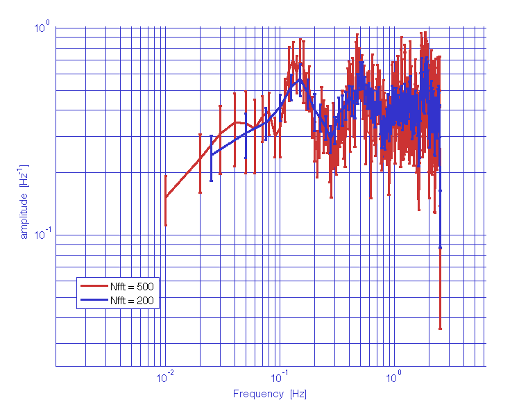
The following example compares the sample variance computed by ao/psd with two different segment length.
% create white noise AO
pl = plist('nsecs', 500, 'fs', 5, 'tsfcn', 'randn(size(t))');
a = ao(pl);

% compute psd with different Nfft
b1 = psd(a, plist('Nfft', 500));
b1.setName('Nfft = 500');
b2 = psd(a, plist('Nfft', 200));
b2.setName('Nfft = 200');

% plot with errorbars
iplot(b1,b2,plist('YErrU',{b1.dy,b2.dy}))
| |
Using spectral windows | Power spectral density estimates | |
©LTP Team