LTPDA Toolbox™

Power spectral density estimates

Description

The LTPDA method ao/psd estimates the power spectral density of time-series signals, included in the input aos following the Welch's averaged, modified periodogram method [1]. Data are windowed prior to the estimation of the spectrum, by multiplying it with a spectral window object, and can be detrended by a polinomial of time in order to reduce the impact of the border discontinuities. The window length is adjustable to shorter lenghts to reduce the spectral density uncertainties, and the percentage of subsequent window overlap can be adjusted as well. The detrending is performed on the individual windows. The user can choose the quantity being given in output among ASD (amplitude spectral density), PSD (power spectral density), AS (amplitude spectrum), and PS (power spectrum).

Syntax

    
    bs = psd(a1, a2, a3, ..., pl)
    bs = psd(as, pl)
    bs = as.psd(pl)

a1, a2, a3, ... are ao(s) containing the input time series to be evaluated. bs includes the output object(s) and pl is an optional parameter list.

Parameters

The parameter list pl includes the following parameters:

'Nfft' - number of samples in each fft [default: length of input data] A string value containing the variable 'fs' can also be used, e.g., plist('Nfft', '2*fs')
'Win' - the window to be applied to the data to remove the discontinuities at edges of segments. [default: taken from user prefs].
The window is described by a string with its name and, only in the case of Kaiser window, the additional parameter 'psll'.
For instance: plist('Win', 'Kaiser', 'psll', 200).
'Olap' - segment percent overlap [default: -1, (taken from window function)]
'Scale' - scaling of output. Choose from:
- 'ASD' - amplitude spectral density
- 'PSD' - power spectral density [default]
- 'AS' - amplitude spectrum
- 'PS' - power spectrum
'Order' - order of segment detrending
- -1 - no detrending
- 0 - subtract mean [default]
- 1 - subtract linear fit
- N - subtract fit of polynomial, order N
'Navs' - number of averages. If set, and if Nfft was set to 0 or -1, the number of points for each window will be calculated to match the request. [default: -1, not set]
'Times' - interval of time to evaluate the calculation on. If empty [default], it will take the whole section.

The length of the window is set by the value of the parameter 'Nfft', so that the window is actually built using only the key features of the window: the name and, for Kaiser windows, the psll.

As an alternative to setting the number of points 'Nfft' in each window, it's possible to ask for a given number of PSD estimates by setting the 'Navs' parameter, and the algorithm takes care of calculating the correct window length, according to the amount of overlap between subsequent segments.

If the user doesn't specify the value of a given parameter, the default value is used.

Algorithm

The algorithm is based in standard MATLAB's tools, as the ones used by pwelch. However, in order to compute the standard deviation of the mean for each frequency bin, the averaging of the different segments is performed using Welford's algorithm [2] which allows to compute mean and variance in one loop.

Examples

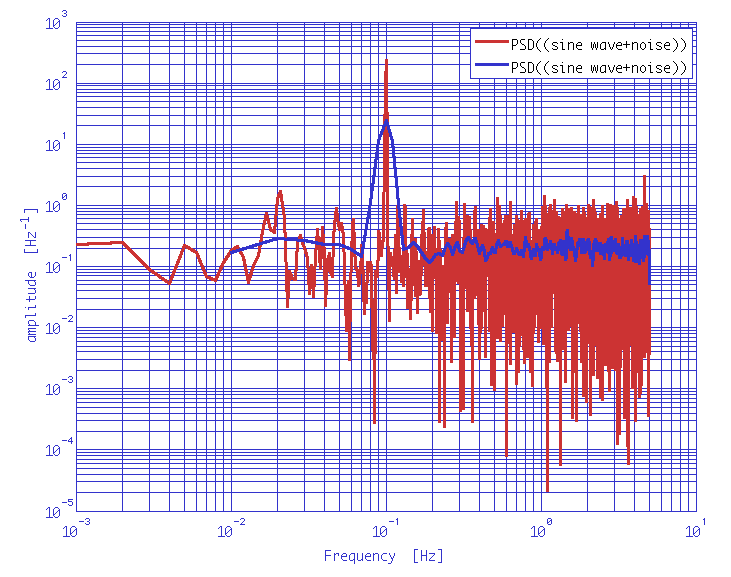
1. Evaluation of the PSD of a time-series represented by a low frequency sinewave signal, superimposed to white noise. Comparison of the effect of windowing on the estimate of the white noise level and on resolving the signal.

    
    % create two AOs
    x1   = ao(plist('waveform','sine wave','f',0.1,'A',1,'nsecs',1000,'fs',10)); 
    x2   = ao(plist('waveform','noise','type','normal','nsecs',1000,'fs',10));
    % add both AOs
    x    = x1 + x2;
    % compute the psd changing the 'nfft'
    y_lf = psd(x);
    y_hf = psd(x,plist('nfft',1000));
    % compare 
    iplot(y_lf, y_hf)

2. Evaluation of the PSD of a time-series represented by a low frequency sinewave signal, superimposed to white noise and to a low frequency linear drift. In the example, the same spectrum is computed with different spectral windows.

    
    % create three AOs
    x1 = ao(plist('waveform','sine wave','f',0.1,'A',1,'nsecs',1000,'fs',10,'yunits','m')); 
    x2 = ao(plist('waveform','noise','type','normal','nsecs',1000,'fs',10,'yunits','m'));
    x3 = ao(plist('tsfcn', 't.^2 + t','nsecs',1000,'fs',10,'yunits','m')); 
    % add them
    x = x1 + x2 + x3;
    % compute psd with different windows
    y_1 = psd(x,plist('scale','ASD','order',1,'win','BH92'));
    y_2 = psd(x,plist('scale','ASD','order',2,'win','Hamming'));
    y_3 = psd(x,plist('scale','ASD','order',2,'win','Kaiser','psll',200));
    % compare
    iplot(y_1, y_2, y_3);

References

P.D. Welch, The Use of Fast Fourier Transform for the Estimation of Power Spectra: A Method Based on Time Averaging Over Short, Modified Periodograms, IEEE Trans. on Audio and Electroacoustics, Vol. 15, No. 2 (1967), pp. 70 - 73.
B. P. Weldford, Note on a Method for Calculating Corrected Sums of Squares and Products, Technometrics, Vol. 4, No. 3 (1962), pp 419 - 420.