LTPDA Toolbox™

contents

Log-scale cross coherence density estimates

Description

The LTPDA method ao/lcohere estimates the coherence function of time-series signals, included in the input aos following the LPSD algorithm [1]. Spectral density estimates are not evaluated at frequencies which are linear multiples of the minimum frequency resolution 1/T, where T is the window lenght, but on a logarithmic scale. The algorithm takes care of calculating the frequencies at which to evaluate the spectral estimate, aiming at minimizing the uncertainty in the estimate itself, and to recalculate a suitable window length for each frequency bin.

Data are windowed prior to the estimation of the spectrum, by multiplying it with a spectral window object, and can be detrended by polinomial of time in order to reduce the impact of the border discontinuities. Detrending is performed on each individual window. The user can choose the quantity being given in output among ASD (amplitude spectral density), PSD (power spectral density), AS (amplitude spectrum), and PS (power spectrum).

Syntax

    
    b = lcohere(a1,a2,pl)
  

a1 and a2 are the 2 aos containing the input time series to be evaluated, b is the output object and pl is an optional parameter list.

Parameters

The parameter list pl includes the following parameters:

• 'Kdes' - desired number of averages [default: 100]
• 'Jdes' - number of spectral frequencies to compute [default: 1000]
• 'Lmin' - minimum segment length [default: 0]
• 'Win' - the window to be applied to the data to remove the discontinuities at edges of segments. [default: taken from user prefs].
  The window is described by a string with its name and, only in the case of Kaiser window, the additional parameter 'psll'.
  For instance: plist('Win', 'Kaiser', 'psll', 200).
• 'Olap' - segment percent overlap [default: -1, (taken from window function)]
• 'Order' - order of segment detrending
  • -1 - no detrending
  • 0 - subtract mean [default]
  • 1 - subtract linear fit
  • N - subtract fit of polynomial, order N
• 'Type' - type of scaling of the coherence function. Choose between:
• 'C' - Complex Coherence Sxy / sqrt(Sxx * Syy) [default ]
• 'MS' - Magnitude-Squared Coherence (abs(Sxy))^2 / (Sxx * Syy)

The function makes magnitude-squadred coherence estimates between the 2 input aos, on a logaritmic frequency scale. If passing two identical objects ai or linearly combined signals, the output will be 1 at all frequencies.

Algorithm

The algorithm is implemented according to [1]. The standard deviation of the mean is computed according to [2]:

is the coherence function. In the LPSD algorithm, the first frequencies bins are usually computed using a single segment containing all the data. For these bins, the sample variance is set to Inf.

Example

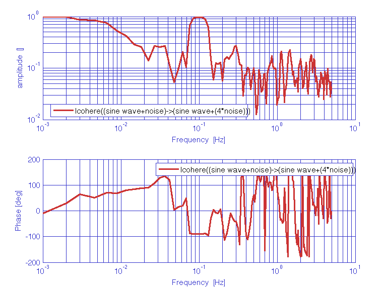
Evaluation of the coherence of two time-series represented by: a low frequency sinewave signal superimposed to white noise, and a low frequency sinewave signal at the same frequency, phase shifted and with different amplitude, superimposed to white noise.

    
    % Parameters
    nsecs = 1000;
    fs  = 10;
    x = ao(plist('waveform','sine wave','f',0.1,'A',1,'nsecs',nsecs,'fs',fs)) + ...
        ao(plist('waveform','noise','type','normal','nsecs',nsecs,'fs',fs));
    x.setYunits('m');
    y = ao(plist('waveform','sine wave','f',0.1,'A',2,'nsecs',nsecs,'fs',fs,'phi',90)) + ...
        4*ao(plist('waveform','noise','type','normal','nsecs',nsecs,'fs',fs));
    y.setYunits('V');
    
    % Compute log coherence
    Cxy = lcohere(x,y,plist('win','Kaiser','psll',200));

    % Plot
    iplot(Cxy);
  

References

1. M. Troebs, G. Heinzel, Improved spectrum estimation from digitized time series on a logarithmic frequency axis, Measurement, Vol. 39 (2006), pp. 120 - 129. See also the Corrigendum.
2. G.C. Carter, C.H. Knapp, A.H. Nuttall, Estimation of the Magnitude-Squared Coherence Function Via Overlapped Fast Fourier Transform Processing , IEEE Trans. on Audio and Electroacoustics, Vol. 21, No. 4 (1973), pp. 337 - 344.

Log-scale cross-spectral density estimates

Log-scale transfer function estimates

©LTP Team