

| LTPDA Toolbox™ | contents | |
The idea of the second exercise is the following:
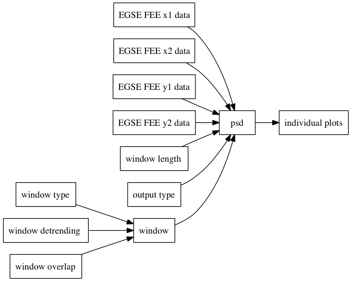
In a flow diagram, the representation is as follows:
The step of building aos by loading data from files was touched upon in previous steps and in the user manual. Here we go ahead by calling the ao constructor method, that we want to specify by means of a plist, with parameters:
| Key | Value | Description |
|---|---|---|
|
FILENAME |
'topic3/EGSE_FEE_x1.dat' |
The name of the file to read the data from. |
|
TYPE |
'tsdata' |
Interpret the data in the file as time-series data. |
|
COLUMNS |
[1 2] |
Load the data x-y pairs from columns 1 (as x) and 2 (as y). |
|
XUNITS |
's' |
Set the units of the x-data to seconds (s). |
|
YUNITS |
'F' |
Set the units of the y-data to farad (F). |
|
COMMENT_CHAR |
'%' |
Indicateds which header lines to skip in the ASCII data file. |
|
FS |
[] |
Indicates to load time series from the first data column. |
|
ROBUST |
'yes' |
Use robust data reading for this file format. |
|
DESCRIPTION |
'EGSE FEE x1 data' |
Set some text to the 'description' field of the AO. |
This procedure can be repeated for all 4 channels we want to analyze, just by calling the ao method and the plist/pset method:
    FEE_x1 = ao(pl_data);
    FEE_x2 = ao(pl_data.pset('FILENAME', 'topic3/EGSE_FEE_x2.dat'));
    FEE_y1 = ao(pl_data.pset('FILENAME', 'topic3/EGSE_FEE_y1.dat'));
FEE_y2 = ao(pl_data.pset('FILENAME', 'topic3/EGSE_FEE_y2.dat'));Now let's proceed by adding the psd step to the diagram, as we did previously. Here we want to call the method only once, without the need of calling the function 4 times; we also want to be sure to apply the same parameters to all the input objects. There are different ways to achieve this; one possibility is to take advantage of the multiple input handling allowed by the ao/psd method. So we go ahead and add pass all the inputs to the psd method:
[S_x1, S_x2, S_y1, S_y2] = psd(FEE_x1, FEE_x2, FEE_y1, FEE_y2);
The spectral leakage is different with different windows. In order to choose the proper one for our needs, we can use the specwin helper, to visualize the window object both in time-domain and frequency domain.

Once we are happy with the choice, we can go apply it to the data, by specifying the value for the Key Win via a parameter list for the psd. One parameter is alreay selected, based on the user preferences. Here I choose to use the Blackman-Harris window, called 'BH92'.
pl_psd = plist('win', 'BH92');
|
The length of the specwin object is irrelevant, because it will be ignored by the psd method, that will rebuild the window only based on the definition (the name). The effective window length is decided by setting the "Nfft" parameter! |
In order to reduce the variance in the estimated PSD, the user may decide to split the input data objects into shorter segments, estimate the fft of the individual segments and then average them. This is set by the "Nfft" parameter. A value of -1 will mean one single window.
Let's choose a window length of 20000 points (2000 seconds at 10 Hz):
pl_psd.pset('nfft', 2e4);In principle, we can decide the amount of overlap among consecutive windows, by entering a percentage value. Let's do nothing here (meaning we leave the default values of -1) and let the psd use the reccomended value which is stored inside the window object and shown as "Rov".
We can decide to give as an output directly the 'ASD' (Amplitude Spectral Density), rather than the 'PSD' (Power Spectral Density). We can also have 'AS' (Amplitude Spectrum) or 'PS' (Power Spectrum). Here I choose to use ASD, so I set the value corresponding to the "Scale" entry to be the 'ASD'.
pl_psd.pset('scale', 'ASD');
Detrending here refers to an additional detrending performed for each individual segment, prior to applying the window. In this case we want to subtract a linear drift, so let's just enter 1 for the value of the key "Order".
pl_psd.pset('order', 1);We can now go ahead and call the method. In this case, since we pass multiple inputs, we can decide what to do with the outputs (we will get one output AO per input AO). Let's keep all of them into a single array:
S = psd(FEE_x1, FEE_x2, FEE_y1, FEE_y2, pl_psd);
As per our choice, psd would give as an output an array of aos corresponding to each input. So in our case, we'd have an array with 4 aos. We can also make them individuals, by indexing the array:
S_x1 = S(1);
We can now go ahead and plot the individual aos in many plots, just by calling iplot. We can also define parameters for each plot, such as colors an so on. Just to exercise let's set the colors to:
| Object | Color |
|---|---|
|
x1 data PSD |
{[1 0 0]} |
|
x2 data PSD |
{[0 1 0]} |
|
y1 data PSD |
{[0 0 1]} |
|
y2 data PSD |
{[1 1 1]} |
At the end we can look at the output plots and check the results, the units, the frequency range.
Once we obtained the objects we are interested on, we can go ahead and save at least the x1 data as described here and here.
| |
Example 1: Simply PSD | Example 3: Log-scale PSD on MDC1 data | |
©LTP Team