LTPDA Toolbox™

Example 1: Simply PSD

The idea of the first exercise is the following:

simulate a time-series of white noise data
evaluate the Power Spectrum of the data
calculate the square root of the calculated power spectrum
plot the results

In a flow diagram, the representation is as follows:

Simulate a time-series of white noise data

There are many different ways to simulate a white noise time series data. Here we choose a pretty powerful one: the "From Waveform" AO constructor.

Let's start building a plist to tune the parameters of the ao constructor: among the available constructor methods, we choose the noise generator via the key WAVEFORM assigning the value "noise". Then let's make the time series last longer by setting the number of seconds (nsecs) to 1000.

    pl_noise  = plist('waveform', 'noise', 'fs', 1, 'nsecs', 1000);

Eventually, we set the units of the noise to be meters by selecting means of the plist method pset: the "Yunits" parameter and entering 'm'.

    pl_noise.pset('yunits', 'm');

To actually build the time-series AO, we then call the ao constructor with the plist we just prepared:

    n = ao(pl_noise);

Evaluate the Power Spectrum of the data

The next step is to choose the parameters for the psd method of the ao class. In order to know the key name, the description, the default and possible values for the parameters, we can type

    help ao/psd

and then click the "Parameters Description" link. Let's discuss the parameters and their meaning:

Nfft allows to choose the number of samples in each periodogram evaluation
Win allows to choose the type of spectral window to be employed to reduce the edge effects at beginning/end of the data sections.
Psll allows to choose the peak-sidelobe level in the case of Kaiser windows.
Olap allows to choose the percentual overlap between subsequent segments
Order allows to choose the degree of detrending applied to each segment prior to windowing
Navs allows to choose the number of averages to perform for each ferquency bin
Times allows to choose a reduced set of the inputs by asking the are within a given time range
Scale allows to choose the quantity to be sent in output (ASD, PSD, AS, PS)

If the user does not specify any value for the parameters, the routine applies the default values.

In this case, we will use the default parameters:

Nfft -1 so to estimate the PSD only on one window, including the whole data set
Win = The value set by the user in the preferences
Psll = 200 in the case of Kaiser window
Olap = -1 so the overlap will be chosen based on the windows properties
Order = 0 so to remove the mean value from the data before applying the window
Navs = -1 so to set the lenght of the window (all data, in this case) rather than asking for a given number of means at each frequency
Times = [] so to analyze all the input data
Scale = 'PSD' so we evaluate the Power Spectral Density [output units] will be [input units]^2 / Hz

In this case, we would not need any specification plist, but let's prepare one. The we can go ahead and do the calculation:

    pl_psd = plist('Scale', 'PSD');
    s = psd(n, pl_psd);

Extract the square root of the calculated power spectrum

For this exercise, we proceed by computing the square root of the calculated spectrum. Notice: by default, as described in its help, ao/sqrt applied to fsdata and tsdata objects acts only on the y (dependent) variable. We'll see later that is possible to choose different outputs for the ao/psd method so as to avoid this step, if we wanted to, by selecting the "Value" 'ASD' for the "Key" 'Scale'.

For now, let's add the sqrt step to the flow by applying it to the output of the ao/psd method.

    a = sqrt(s);

Plot the results

What remains is just to plot the calculated square root of the PSD of the input white noise. Just call ao/iplot. The output one should be similar to the following:

PSD 1: evaluated PSD

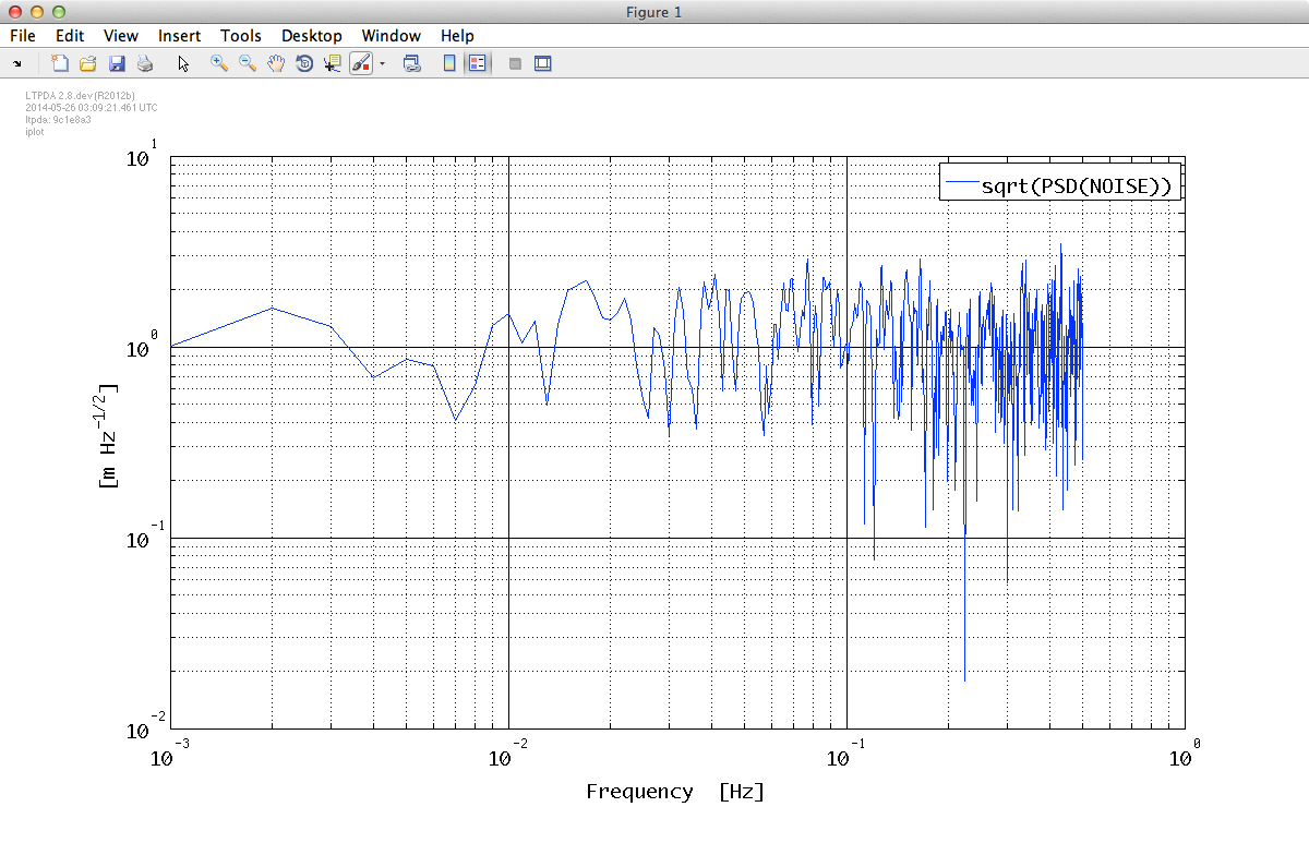
Please notice:

The log-log shape of the plot
The x-axis units
The y-axis units
The history steps reported on the legend

Power Spectral Density estimation

Example 2: Windowing data