

| LTPDA Toolbox™ | contents | |
Analysis objects can be created in MATLAB in many ways. Apart from being created by the many algorithms in the LTPDA Toolbox, AOs can also be created from initial data or descriptions of data. The various constructors are listed in the function help: ao help.
The following examples show some ways to create Analysis Objects.
Analysis Objects can be created from text files containing ASCII numbers. Files ending in '.txt' or '.dat' will be handled as ASCII file inputs. The first column is taken to be the amplitude samples. The created AO is of type cdata. The following code shows this in action:
       >>  a = ao('data.txt')
Warning: !!! You haven't defined a data type.
The output will be an AO with constant data.
> In ao.fromDatafile at 75
  In ltpda_uo.fromFile at 157
  In ao.ao>ao.ao at 348
----------- ao 01: a -----------

       name: ''
       data: 0 0.1 0.2 0.3 0.4 0.5 0.6 0.7 0.8 0.9 ...
             -------- cdata [vals] ------------
                  y:  [100x2], double
                 dy:  [0x0], double
             yunits:
             ----------------------------------

       hist: ao / ao / 11c33bf1421898d27b94853f646e22673ebc750d
description:
       UUID: 714712ad-dcbf-48dc-b453-124bc401cfc3
--------------------------------
As with most constructor calls, an equivalent action can be achieved using an input Parameter List.
>> a = ao(plist('filename', 'data.txt'))
A very useful constructor for the user is the following: the first column is taken to be the time instances; the second column is taken to be the amplitude samples. The created AO is of type tsdata with the sample rate set by the difference between the time-stamps of the first two samples in the file. The name of the resulting AO is set to the filename (without the file extension). The filename is also stored as a parameter in the history parameter list. In order to obtain this, the ao constructor needs to be configured via a plist:
        >> a = ao('data.txt', plist('type', 'tsdata', 'columns', [1 2]))
----------- ao 01: a -----------

       name: ''
       data: (0,-1.57598732060313) (0.1,1.82575122802555) (0.2,0.204267478815429) (0.3,-1.16339579241533) (0.4,0.120609818645024) ...
             -------- tsdata [x, y] --------

                  x:  [100 1], double
                  y:  [100 1], double
                 dx:  [0 0], double
                 dy:  [0 0], double
             xunits:  [s]
             yunits:
                  fs:  10
               nsecs:  10
                  t0:  1970-01-01 00:00:00.000 UTC
             -------------------------------

       hist: ao / ao / 11c33bf1421898d27b94853f646e22673ebc750d
description:
       UUID: 467d68e1-0a0a-4f9d-928a-536a74427f31
--------------------------------
AOs can be saved as both XML and .MAT files. As such, they can also be created from these files.
        >> a = ao('a.xml')
        ----------- ao 01: a -----------

       name: ''
       data: (0,-1.57598732060313) (0.1,1.82575122802555) (0.2,0.204267478815429) (0.3,-1.16339579241533) (0.4,0.120609818645024) ...
             -------- tsdata [x, y] --------

                  x:  [100 1], double
                  y:  [100 1], double
                 dx:  [0 0], double
                 dy:  [0 0], double
             xunits:  [s]
             yunits:
                  fs:  10
               nsecs:  10
                  t0:  1970-01-01 00:00:00.000 UTC
             -------------------------------

       hist: ao / ao / 11c33bf1421898d27b94853f646e22673ebc750d
description:
       UUID: 467d68e1-0a0a-4f9d-928a-536a74427f31
--------------------------------
AOs can be created from any valid MATLAB function which returns a vector or matrix of values. For such calls, a parameter list is used as input. For example, the following code creates an AO containing 1000 random numbers:
        >> a = ao(plist('fcn', 'randn(1000, 1)'))
        ----------- ao 01: a -----------

       name: ''
       data: 0.0704977862099333 -1.93302660372422 0.818722013821727 1.26175710906169 1.16734286458427 -0.570329994878025 -0.393897571578092 -1.01743401819165 0.250205871646325 0.252124808964812 ...
             -------- cdata [vals] ------------
                  y:  [1000x1], double
                 dy:  [0x0], double
             yunits:
             ----------------------------------

       hist: ao / ao / 11c33bf1421898d27b94853f646e22673ebc750d
description:
       UUID: 9744572a-349c-4ed5-bb12-26cee0a2c6c6
--------------------------------
Here you can see that the AO is a cdata type.
The name of the AOs can be created when building the objects, via the name parameter:
        >> a = ao(plist('fcn', 'randn(1000, 1)', 'name', 'My data'))
        ----------- ao 01: My data -----------

       name: My data
       data: -0.00551290141704299 1.20011431909571 -1.03401713888056 -0.847567754466168 0.433422036872966 -0.887523979425756 0.121232620802761 -0.401904890482745 1.09667832321064 0.436674648218274 ...
             -------- cdata [vals] ------------
                  y:  [1000x1], double
                 dy:  [0x0], double
             yunits:
             ----------------------------------

       hist: ao / ao / 11c33bf1421898d27b94853f646e22673ebc750d
description:
       UUID: 41adbb93-abb9-42bb-843a-62e26d7f3729
--------------------------------------
AOs can be created from any valid MATLAB function which is a function of the variable t. For such calls, a parameter list is used as input. For example, the following code creates an AO containing sinusoidal signal at 1Hz with some additional Gaussian noise:
        pl = plist();
        pl = append(pl, 'nsecs', 100);
        pl = append(pl, 'fs', 10);
        pl = append(pl, 'tsfcn', 'sin(2*pi*1*t)+randn(size(t))');
        a = ao(pl)
        ----------- ao 01: a -----------

       name: ''
       data: (0,1.2598690621946) (0.1,-0.518094254597338) (0.2,1.01242966287229) (0.3,2.18175020239501) (0.4,1.13289098425403) ...
             -------- tsdata [x, y] --------

                  x:  [1000 1], double
                  y:  [1000 1], double
                 dx:  [0 0], double
                 dy:  [0 0], double
             xunits:  [s]
             yunits:
                  fs:  10
               nsecs:  100
                  t0:  1970-01-01 00:00:00.000 UTC
             -------------------------------

       hist: ao / ao / 11c33bf1421898d27b94853f646e22673ebc750d
description:
       UUID: 4d8d5a69-1fd8-4638-8afd-02d1e42cb951
--------------------------------
Here you can see that the AO is a tsdata type, as you would expect. Also note that you need to specify the sample rate (fs) and the number of seconds of data you would like to have (nsecs).
The LTPDA Toolbox contains a class for designing spectral windows (see Spectral Windows). A spectral window object can also be used to create an Analysis Object as follows:
        >> w = specwin('Hanning', 1000)
        ------ specwin/1 -------
      type: Hanning
     alpha: 0
      psll: 31.5
       rov: 50
     nenbw: 1.5
      w3db: 1.4381999999999999
  flatness: -1.4236
levelorder: []
      skip: 0
       len: 1000
------------------------

        >> a = ao(w)
        ----------- ao 01: ao(Hanning) -----------

       name: ao(Hanning)
       data: 0 9.86957193144233e-06 3.94778980919441e-05 8.88238095955174e-05 0.00015790535835003 0.0002467198171342 0.000355263679705398 0.000483532660937647 0.000631521696991266 0.000799224945512489 ...
             -------- cdata [vals] ------------
                  y:  [1x1000], double
                 dy:  [0x0], double
             yunits:
             ----------------------------------

       hist: ao / ao / 11c33bf1421898d27b94853f646e22673ebc750d
description:
       UUID: 44686f99-9426-43da-8adf-73d092254c05
------------------------------------------
It is also possible to pass the information about the window as a plist to the ao constructor.
        >> ao(plist('win', 'Hanning', 'length', 1000))
        ----------- ao 01: ao(Hanning) -----------

       name: ao(Hanning)
       data: 0 9.86957193144233e-06 3.94778980919441e-05 8.88238095955174e-05 0.00015790535835003 0.0002467198171342 0.000355263679705398 0.000483532660937647 0.000631521696991266 0.000799224945512489 ...
             -------- cdata [vals] ------------
                  y:  [1x1000], double
                 dy:  [0x0], double
             yunits:
             ----------------------------------

       hist: ao / ao / 11c33bf1421898d27b94853f646e22673ebc750d
description:
       UUID: 02b145c2-ae2f-40af-a149-53b66ed06d58
------------------------------------------
The example code above creates a Hanning window object with 1000 points. The call to the AO constructor then creates a cdata type AO with 1000 points. This AO can then be multiplied against other AOs in order to window the data.
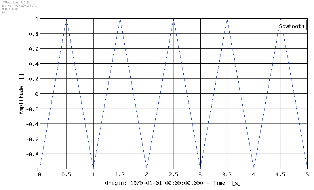
MATLAB contains various functions for creating different waveforms, for example, square, sawtooth. Some of these functions can be called upon to create Analysis Objects. The following code creates an AO with a sawtooth waveform:
        pl = plist();
        pl = append(pl, 'fs', 100);
        pl = append(pl, 'nsecs', 5);
        pl = append(pl, 'waveform', 'Sawtooth');
        pl = append(pl, 'f', 1);
        pl = append(pl, 'width', 0.5);

        asaw = ao(pl)
        ----------- ao 01: Sawtooth -----------

       name: Sawtooth
       data: (0,-1) (0.01,-0.96) (0.02,-0.92) (0.03,-0.88) (0.04,-0.84) ...
             -------- tsdata [x, y] --------

                  x:  [1 500], double
                  y:  [1 500], double
                 dx:  [0 0], double
                 dy:  [0 0], double
             xunits:  [s]
             yunits:
                  fs:  100
               nsecs:  5
                  t0:  1970-01-01 00:00:00.000 UTC
             -------------------------------

       hist: ao / ao / 11c33bf1421898d27b94853f646e22673ebc750d
description:
       UUID: fd01eb6e-4a93-4c5a-be8b-77efa23da2d1
---------------------------------------
You can call the iplot function to view the resulting waveform:
iplot(asaw);
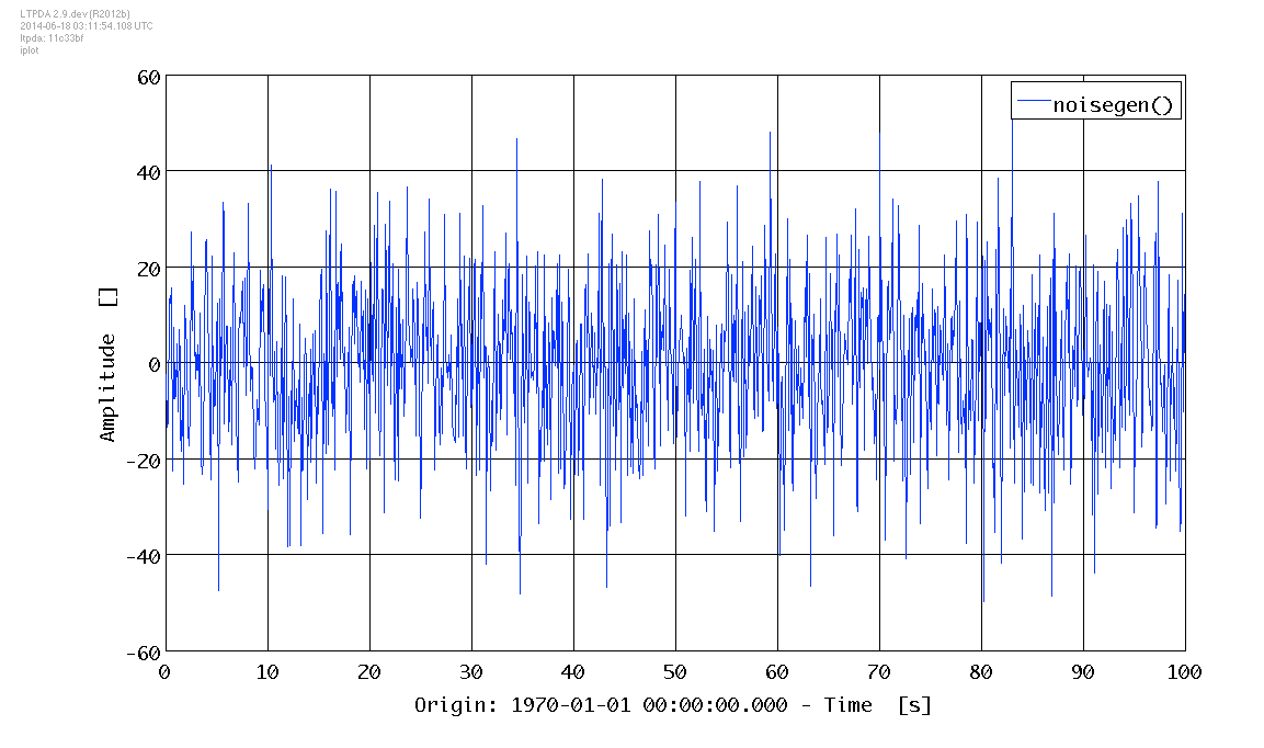
When generating an AO from a pole zero model, the noise generator function is called. This a method to generate arbitrarily long time series with a prescribed spectral density. The algorithm is based on the following paper:
Franklin, Joel N.: Numerical simulation of stationary and non-stationary gaussian random processes , SIAM review, Volume { 7}, Issue 1, page 68--80, 1965.
The Document Generation of Random time series with prescribed spectra by Gerhard Heinzel (S2-AEI-TN-3034)
corrects a mistake in the aforesaid paper and describes the practical implementation.
The following code creates an AO with a time series having a prescribed spectral density,
defined by the input pole zero model:
	f1    = 5;
	f2    = 10;
	f3    = 1;
	gain  = 1;
	fs    = 10;  % sampling frequancy
	nsecs = 100; % number of seconds to be generated

	p = [pz(f1) pz(f2)];
	z = [pz(f3)];
	pzm = pzmodel(gain, p, z);
	a = ao(pzm, nsecs, fs)
----------- ao 01: noisegen() -----------

       name: noisegen()
       data: (0,-5.76788205447447) (0.1,-2.52555281234382) (0.2,-13.5550152475477) (0.3,-12.3242958095728) (0.4,13.1571973729713) ...
             -------- tsdata [x, y] --------

                  x:  [1000 1], double
                  y:  [1000 1], double
                 dx:  [0 0], double
                 dy:  [0 0], double
             xunits:  [s]
             yunits:
                  fs:  10
               nsecs:  100
                  t0:  1970-01-01 00:00:00.000 UTC
             -------------------------------

       hist: ao / ao / 11c33bf1421898d27b94853f646e22673ebc750d
description:
       UUID: 40b52491-4880-4dbc-bb48-46202db99475
-----------------------------------------
You can call the iplot function to view the resulting noise.
iplot(a);
| |
Analysis Objects | Saving Analysis Objects | |
©LTP Team