LTPDA Toolbox™

Example 3: Log-scale PSD on MDC1 data

The idea of the third exercise is the following:

load a time-series of IFO noise data simulated for the first LTPDA Mock Data Challenge (MDC1)
set data units
evaluate the Log-Scale Power Spectrum of the 2 IFO channels data
set the plot properties
plot the results

In a flow diagram, the representation is as follows:

Load a time-series of IFO noise data simulated for the first LTPDA Mock Data Challenge (MDC1)

The step of building aos by loading data from files was touched upon in previous steps and in the user manual. Here we go ahead by calling the ao constructor method, that we want to specify by means of a plist, with parameters:

Key	Value	Description
`FILENAME`	'topic3/mockdata_16_48_17_11_2007_1.dat'	The name of the file to read the data from.
`TYPE`	'tsdata'	Interpret the data in the file as time-series data.
`COLUMNS`	[1 2 1 3]	Load the data x-y pairs from columns 1 (as x) and 2 (as y), in the first `ao`, and from columns 1 (as x) and 3 (as y), in the second `ao`.
`XUNITS`	's'	Set the units of the x-data to seconds (s).
`YUNITS`	''	We leave this empty for now.
`COMMENT_CHAR`	'%'	Indicateds which header lines to skip in the ASCII data file.
`FS`	[]	Indicates to load time series from the first data column.
`ROBUST`	'no'	We don't need robust data reading for these simulated data.
`NAME`	{'IFO x1', 'IFO x12'}	Specify the names of the objects.
`DESCRIPTION`	'MDC1 set #1, 17/11/2007'	Set some text to the 'description' field of the AO.

x = ao(pl_load);

The output will be a vector of aos, containing:

the x1 IFO measurement (SC to TM1 x position)
the x12 IFO measurement (TM2 to TM1 relative x position)

We can then run all the analyses, and be sure to be applying the same parameters, by passing the vector of aos to the various methods.

Set data units

We forgot to set the units ... luckily both displacements are expressed in meters, so let's call the method

ao/setYunits

The relevant parameters to set are:

Key	Value	Description
`YUNITS`	'm'	The unit object to set as y-units

Evaluate the Log-Scale Power Spectrum of the 2 IFO channels data

Now let's go ahead and use the lpsd method on the ao class. It needs to be specified by setting its parameters. Many of these parameters are the same as we already discussed for ao/psd:

Win Allows to choose the type of spectral window to be employed to reduce the edge effects at beginning/end of the data sections.
Olap Allows to choose the percentual overlap between subsequent segments
Order Allows to choose the degree of detrending applied to each segment prior to windowing
Scale Allows to choose the quantity to be sent in output (ASD, PSD, AS, PS)
Times Allows to choose a reduced set of the inputs by asking the are within a given time range

In this case, we will use the following parameters:

Key	Value	Description
`WIN`	'BH92'	Or a different one, if you want.
`OLAP`	-1	Overlap will be chosen based on the window properties
`ORDER`	2	Segment-wise detrending up to order 2
`SCALE`	'ASD'	Evaluate the Amplitude Spectral Density so that [output units] will be [input units] / sqrt(Hz)

We also need to set other 2 parameters that are typical of this method, discussed in the devoted user manual section.

'Jdes' - the number of spectral frequencies to compute
'Kdes' - the desired number of averages
'Lmin' - the minimum segment length [default: 0]

We will act on the first one, so to decide how many ASD bins to estimate, leaving to the algorithm the choice of their location and the length of the windows on each bin.

Key	Value	Description
`JDES`	2000	Compromising execution time and resolution
`KDES`	10	Slightly less than the default value
`LMIN`	0	The default value

Plot the results

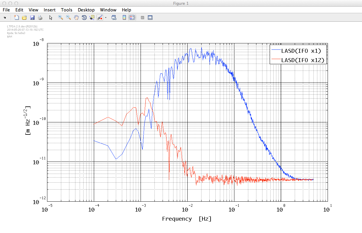
As we did in previous topics, let's add one ao/iplot step after the call to the ao/lpsd method. We make a little additional exercise: let's specify the color via a plist with parameters:

Key	Value	Description
`COLORS`	{[0 0 1],[1 0 0]}	Setting x1 to blue and x12 to red

The execution may take some while ... and here are the results:

Example 2: Windowing data

Empirical Transfer Function estimation