

| LTPDA Toolbox™ | contents | |
Non-linear least square fitting of time-series exploits the function ao/xfit.
During this exercise we will:
Let us open a new editor window and load test data.
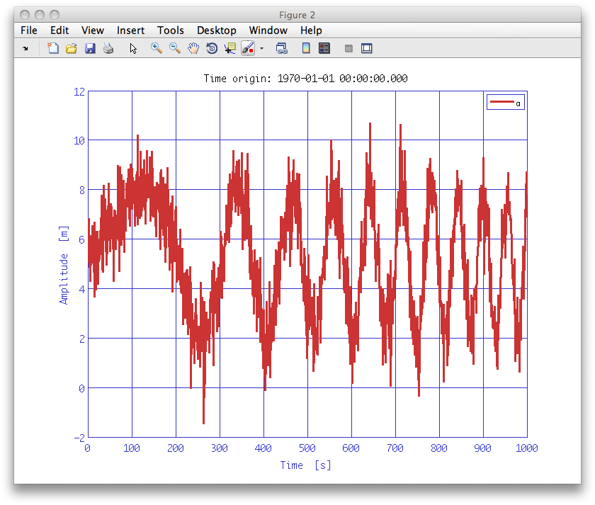
    a = ao(plist('filename', 'topic5/T5_Ex05_TestNoise.xml'));
    a.setName('data');
    iplot(a)
As can be seen this is a chirped sine wave with some noise.
    mdl = smodel(plist('Name', 'chirp', ...
              'expression', 'A.*sin(2*pi*(f + f0.*t).*t + p) + c', ...
              'params', {'A', 'f', 'f0', 'p', 'c'}, ...
              'xvar', 't', ...
              'xunits', 's', 'yunits', 'm'));
    plfit1 = plist('Function', mdl, ...
              'P0', [5, 9e-5, 9e-6, 0, 5]);

    params1 = xfit(a, plfit1);
Once the fit is done, we can evaluate our model to check fit results.
    b = eval(params1, plist('xdata', a, 'xfield', 'x'));
    b.setName();
    iplot(a, b)
As you can see, the fit is not accurate. One of the great problems of non-linear least square methods is that they easily find a local minimum of the chi square function and stop there without finding the global minimum. There are two possibile solutions to such kind of problems: the first one is to refine step by step the fit by looking at the data; the second one is to perform a Monte Carlo search in the parameter space. This way, the fitting machinery extracts the number of points you define in the 'Npoints' key, evaluates the chi square at those points, reoders by ascending chi square, selects the first guesses and fit starting from them.
plfit2 = plist(...
		'Function', mdl, ...
		'MonteCarlo', 'yes', ...
		'Npoints', 1000, ...
		'LB', [1, 5e-5, 5e-6, 0, 2], ...
		'UB', [10, 5e-4, 5e-5, 2*pi, 7]);

    params2 = xfit(a, plfit2);

    c = eval(params2, plist('xdata', a, 'xfield', 'x'));
    c.setName();
    iplot(a, c)
The fit now looks like better...

    A  = 3
    f  = 1e-4
    f0 = 1e-5
    p  = 0.3
    c  = 5
Fitted parameters are instead:
    A  = 3.02 +/- 0.05
    f  = (7 +/- 3)e-5
    f0 = (1.003 +/- 0.003)e-5
    p  = 0.33 +/- 0.04
    c  = 4.97 +/- 0.03
The correlation matrix of the parameters, the chi square, the degree of freedom, the covariance matrix are store in the output pest. Other useful information are stored in the procinfo (processing information) field. This field is a plist and is used to additional information that can be returned from algorithms. For example, to extract the chi square, we write:
    params2.chi2
    1.0253740840052
And to know the correlation matrix:
    params2.corr
    Columns 1 through 3

                         1         0.120986348157139       -0.0970894969803509
         0.120986348157139                         1        -0.966114904879414
       -0.0970894969803509        -0.966114904879414                         1
        -0.156801230958825        -0.848296014553159         0.717376893765734
       -0.0994358284166703         0.187645552903433        -0.169496082635319

    Columns 4 through 5

        -0.156801230958825       -0.0994358284166703
        -0.848296014553159         0.187645552903433
         0.717376893765734        -0.169496082635319
                         1        -0.199286767157984
        -0.199286767157984                         1
Not so bad!
| |
Fitting time series with polynomials | IFO/Temperature Example - signal subtraction | |
©LTP Team