

| LTPDA Toolbox™ | contents | |
During this exercise we will:
Let us load the test data and split out the 'good' part as we did in Topic 3:
    ifo = ao(plist('filename', 'ifo_temp_example/ifo_fixed.xml'));
    ifo.setName();
    T = ao(plist('filename', 'ifo_temp_example/temp_fixed.xml'));
    T.setName();

    % Split out the good part of the data
    pl_split = plist('split_type', 'interval', ...
                'start_time', ifo.t0 + 40800, ...
                'end_time', ifo.t0 + 193500);

    ifo_red = split(ifo, pl_split);
    T_red = split(T, pl_split);
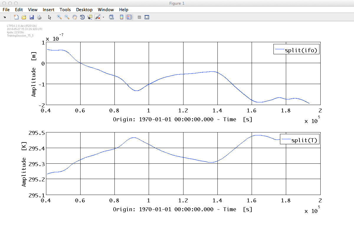
These data are already preprocessed with ao/consolidate in order to set
the sampling frequency to 1Hz.
We could look at the data...
iplot(ifo_red, T_red, plist('arrangement', 'subplots'))
Let us load the transfer function estimate we calculated in Topic 3.
tf = ao('ifo_temp_example/T_ifo_tf.xml');
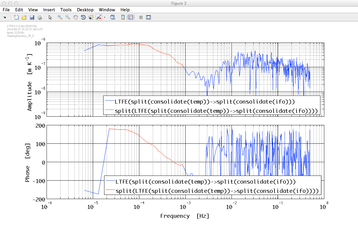
The meaningful frequency region is in the range 2e-5 Hz - 1e-3 Hz. Therefore we split the transfer function to extract only meaningful data.
    tfsp = split(tf, plist('frequencies', [2e-5 1e-3]));
    iplot(tf, tfsp)
The plot compares full range TF with splitted TF:
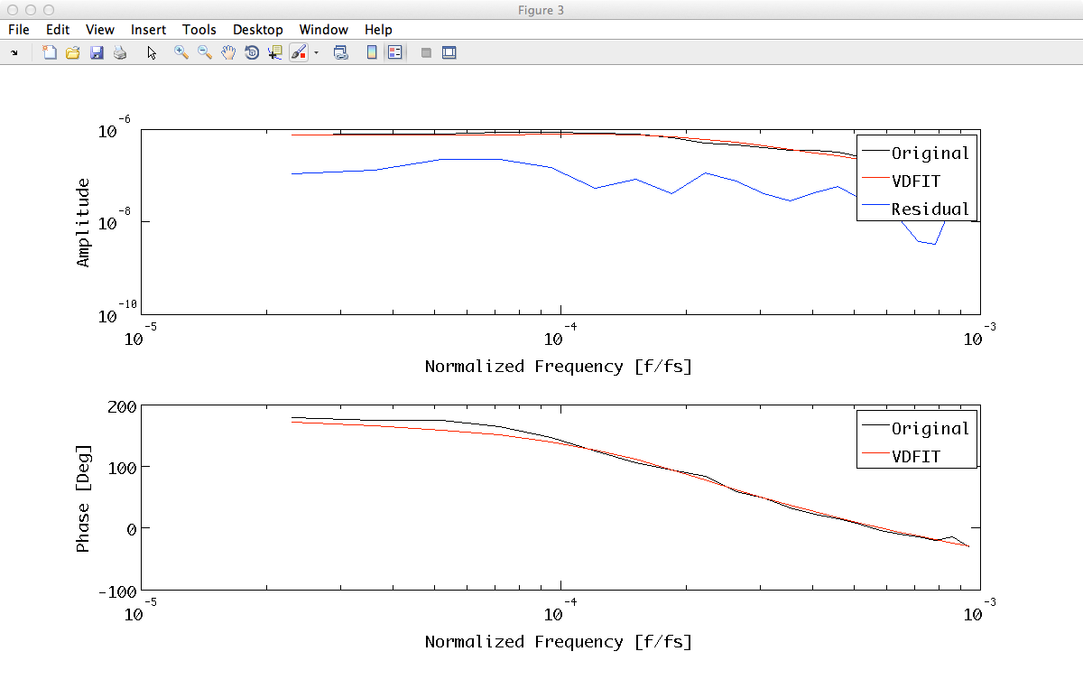
    plfit = plist(...
        'AutoSearch', 'off', ...
        'StartPolesOpt', 'clog', ...
        'maxiter', 5, ...
        'minorder', 3, ...
        'maxorder', 3, ...
        'weightparam', 'abs', ...
        'Plot', 'on', ...
        'ForceStability', 'on', ...
        'CheckProgress', 'off');

    fobj = zDomainFit(tfsp, plfit);
    fobj.filters.setIunits('K');
    fobj.filters.setOunits('m');
It is time to filter temperature data with the fit output in order to extract temperature contribution to interferometer output. Detrend after the filtering is performed to subtract mean to data (bias subtraction).
    ifoT = filter(T, fobj, plist('bank','parallel'));
    ifoT = split(ifoT, pl_split);
    ifoT.detrend(plist('order', 0));
    ifoT.simplifyYunits;
    ifoT.setName();
Then we subtract temperature contribution from measured interferometer data
  ifonT = ifo_red - ifoT;
  ifonT.setName();
The figure reports measured interferometer data, temperature contribution to interferometer output and interferometer output without thermal drifts.
iplot(ifo_red, ifoT, ifonT)

If you now compare spectra of the original IFO signal and the one with the temperature contribution removed, you should see something like the figure below:
  ifoxx = ifo_red.lpsd;
  ifonTxx = ifonT.lpsd;
  iplot(ifoxx, ifonTxx)

| |
Non-linear least squares fitting of time series | LTPDA Training Session 2 | |
©LTP Team