Fitting time series with polynomials (LTPDA Toolbox)

Fitting time series with polynomials exploits the function ao/polyfit. Details on the agorithm can be found in the appropriate help page.

Fitting time series with polynomials

    a = ao(plist('filename', 'topic5/T5_Ex04_TestNoise.xml'));
    a.setName();

Try to fit data with ao/polyfit. We decide to fit with a 6th order polynomial.

    plfit = plist('N', 6);
    p     = polyfit(a, plfit)

The output of the polifit method is a parameter estimation object (pest-object). This object contains the coefficients of the fitted polynomial.

---- pest 1 ----
       name: polyfit(a)
 parameters:
             P1:   9.1738842e-15 +-   5.0781997e-14 [m s^(-6)]
             P2:  -1.0105535e-11 +-   1.5272591e-10 [m s^(-5)]
             P3:   1.1467469e-08 +-   1.7567488e-07 [m s^(-4)]
             P4:  -2.8397623e-06 +-   9.6440306e-05 [m s^(-3)]
             P5:   -0.0044447573 +-     0.025624775 [m s^(-2)]
             P6:      0.13779743 +-       2.9321071 [m s^(-1)]
             P7:       47.519031 +-       105.42745 [m]
 
        pdf: []
        cov: [7x7], ([2.57881118597054e-27 -7.72869712435383e-24 8.77207944145014e-21 -4.67120229268015e-18 1.16517894641315e-15 -1.16052934006908e-13 2.73279821621369e-12;-7.72869712435383e-24 2.33252022407021e-20 -2.66952587411623e-17 1.43594424166059e-14 -3.6267488596848e-12 3.66996931772136e-10 -8.8246258706484e-09;8.77207944145014e-21 -2.66952587411623e-17 3.08616635389935e-14 -1.68087475028813e-11 4.3130451226497e-09 -4.45597417857348e-07 1.10252789031329e-05;-4.67120229268015e-18 1.43594424166059e-14 -1.68087475028813e-11 9.30073263760312e-09 -2.43649023481382e-06 0.00025896803296049 -0.00667866538500405;1.16517894641315e-15 -3.6267488596848e-12 4.3130451226497e-09 -2.43649023481382e-06 0.000656629115560015 -0.0727240078893827 2.0026099434953;-1.16052934006908e-13 3.66996931772136e-10 -4.45597417857348e-07 0.00025896803296049 -0.0727240078893827 8.59725202675112 -266.884491131194;2.73279821621369e-12 -8.8246258706484e-09 1.10252789031329e-05 -0.00667866538500405 2.0026099434953 -266.884491131194 11114.9468971226])
       corr: []
      chain: []
       chi2: 1
        dof: 993
     models: smodel(P1*X.^6 + P2*X.^5 + P3*X.^4 + P4*X.^3 + P5*X.^2 + P6*X.^1 + P7*X.^0)
description: 
       UUID: 08970689-fe18-4581-8040-cff939363a32
----------------

Once we have the pest object with the coefficients, we can evaluate it. In order to construct an object with the same time base we can pass the input AO, and specify to use its 'x' field to build the 'x' field of the output.

    b = p.eval(a, plist('type', 'tsdata', 'xfield', 'x'));
    b.setName();

Now, let's check the fit results with some plotting. We can compare data with fitted model and look at the fit residuals.

    iplot(a, b)
    iplot(a - b)

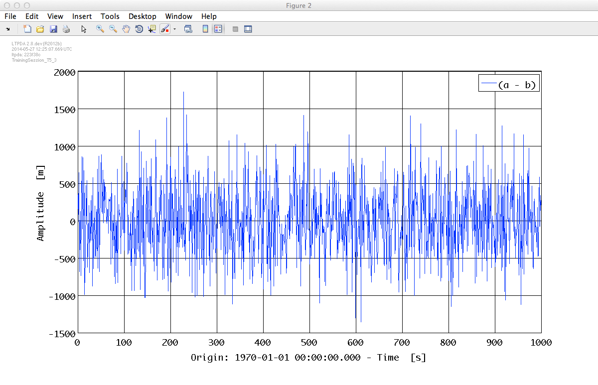
You could also try using ao/detrend on the input time-series to yield a very similar result as that shown in the last plot.