

| LTPDA Toolbox™ | contents | |
System identification in Z-domain is performed with the function ao/zDomainFit. It is based on a modified version of the vector fitting algorithm that was adapted to fit in the Z-domain. Details of the agorithm can be found in the Z-domain fit documentation page.
During this exercise we will:
Let's start by generating some white noise.
a = ao(plist('tsfcn', 'randn(size(t))', 'fs', 1, 'nsecs', 10000, 'yunits', 'm'));
This command generates a time series of gaussian distributed random noise with a sampling frequency ('fs') of 1 Hz, 10000 seconds long ('nsecs') and with 'yunits' set to meters ('m').
Now we are ready to move on the second step where we will:
	% Build a pole-zero model
    pzm = pzmodel(1, [0.005 2], [0.05 4]);

	% Construct a miir filter from the pzmodel
    filt   = miir(pzm, plist('fs', 1, 'name', 'None'));
    filt.setIunits('m');
    filt.setOunits('V');

    % Filter white noise data with the filter in order to obtain a colored noise time series
    ac = filter(a, filt);
    ac.simplifyYunits;
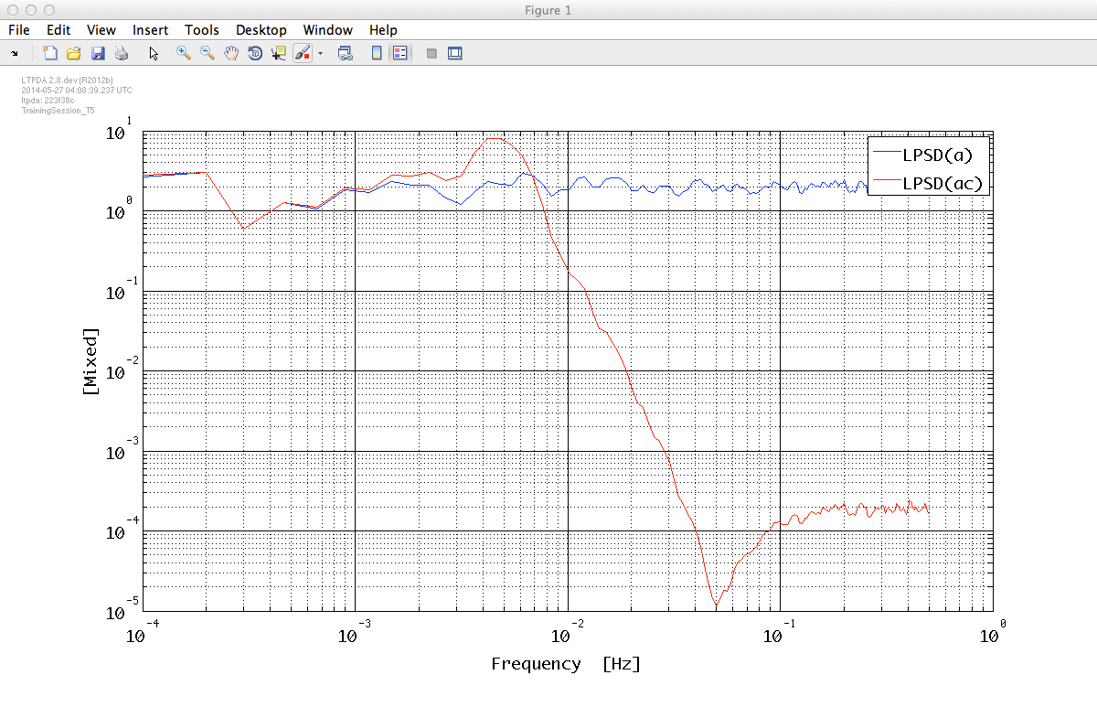
We can calculate the PSD of the data streams in order to check the difference between the coloured noise and the white noise. Let's choose the log-scale estimation method.
    axx  = lpsd(a);
    acxx = lpsd(ac);
    iplot(axx,acxx)
You should obtain a plot similar to this:
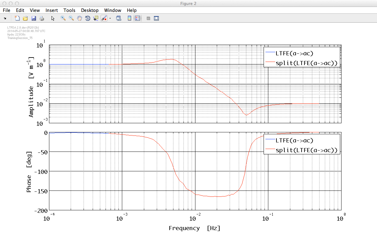
Let us move to the third step. We will generate the transfer function from the data and split it in order to remove the first 3 bins. The last operation is useful for the fitting process.
    tf = ltfe(a, ac);
    tfsp = split(tf, plist('frequencies', [5e-4 5e-1]));

    iplot(tf, tfsp)
The plot should look like the following:
It is now the moment to start fitting with zDomainFit. As reported in the
function help page we can run an automatic search loop to identify the proper model order.
In such a case we have to define a set of conditions to check fit accuracy and to exit the fitting loop.
We can start checking Mean Squared Error and variation (CONDTYPE = 'MSE').
It checks if the normalized mean squared error is lower than the value specified in the parameter FITTOL
and if the relative variation of the mean squared error is lower than the value specified in the parameter MSEVARTOL.
Default |
|||
|---|---|---|---|
| Key | Default Value | Options | Description |
| CONDTYPE | 'MSE' |
|
Fit conditioning type. Admitted values are:
|
| FITTOL | 0.001 | none | Fit tolerance. |
| MSEVARTOL | 0.01 | none | Mean Squared Error Variation - Check if the relative variation of the mean squared error is smaller than the value specified. This option is useful for finding the minimum of the Chi-squared. |
You will find a list of all Parameters of zDomainFit here: Parameter of zDomainFit
Now let's run the fit:
    % Set up the parameters
    plfit = plist('fs', 1, ...      % Sampling frequency for the model filters
      'AutoSearch', 'on', ...       % Automatically search for a good model
      'StartPolesOpt', 'clog', ...  % Define the properties of the starting poles - complex distributed in the unitary circle
      'maxiter', 50 ,...            % Maximum number of iteration per model order
      'minorder', 2, ...            % Minimum model order
      'maxorder', 9, ...            % Maximum model order
      'weightparam', 'abs', ...     % Assign weights as 1./abs(data)
      'condtype', 'MSE', ...        % Mean Squared Error and variation
      'fittol', 1e-2, ...           % Fit tolerance
      'msevartol', 1e-1, ...        % Mean Squared Error Variation tolerance
      'Plot', 'on', ...             % Set the plot on or off
      'ForceStability', 'on', ...   % Force to output a stable poles model
      'CheckProgress', 'off');      % Display fitting progress on the command window

    % Do the fit
    fobj = zDomainFit(tfsp, plfit);

    % Set the input and output units for fitted model
    fobj.setIunits('m');
    fobj.setOunits('V');
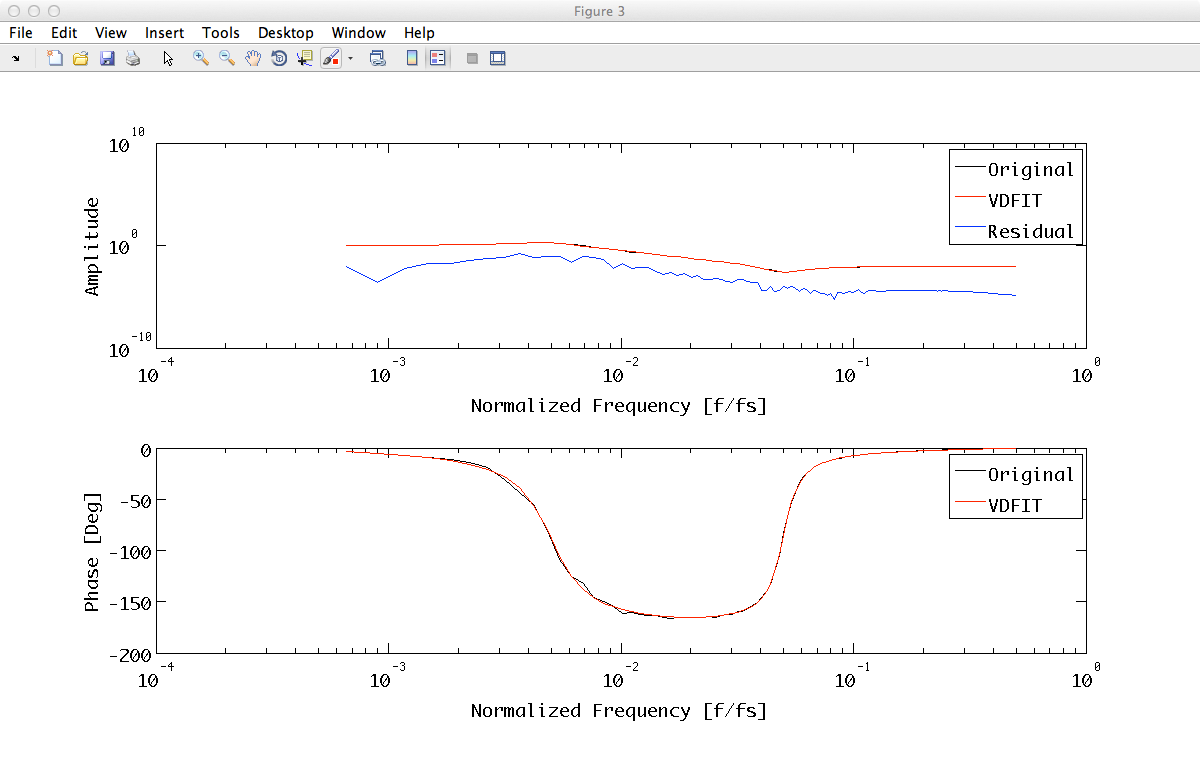
When 'Plot' parameter is set to 'on' the function plots the fit progress.
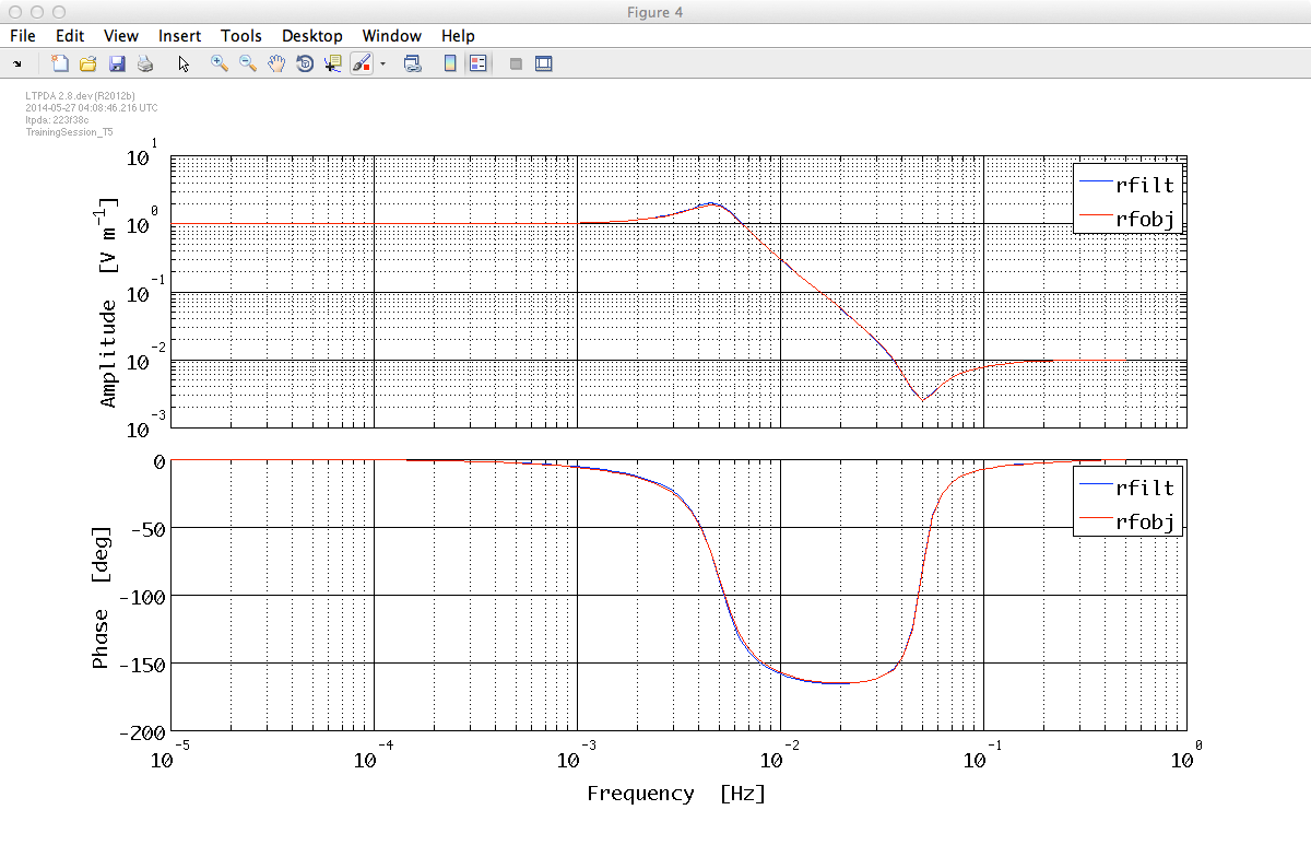
We can now check the result of our fitting procedures. We calculate the frequency response of the fitted models (filters) and compare them with the starting IIR filter response, then we will plot the percentage error on the filters magnitudes.
Note that the result of the fitting procedure is a matrix object containing a filterbank object, which itself contains a parallel bank of 3 IIR filters.
Note that at the moment we need to access the individual filter objects inside the matrix object that was the result of the fitting procedure.
% set plist for filter response
plrsp = plist('bank', 'parallel', 'f1', 1e-5, 'f2', 0.5, 'nf', 100, 'scale', 'log');
% compute the response of the original noise-shape filter
rfilt = resp(filt, plrsp);
rfilt.setName;
% compute the response of our fitted filter bank
rfobj = resp(fobj.filters, plrsp);
rfobj.setName;
% compare the responses
iplot(rfilt, rfobj)
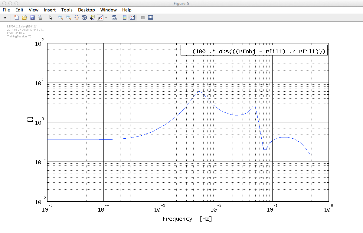
% and the percentage error on the magnitude
pdiff = 100 .* abs((rfobj - rfilt) ./ rfilt);
pdiff.simplifyYunits;
iplot(pdiff, plist('YRanges', [1e-2 100]))
The first plot shows the response of the original filter and the fitted filter bank,
whereas the second plot reports the percentage difference between fitted model and target filter magnitude.
As can be seen, the difference between filters magnitude is at most 10%.
| |
Topic 5 - Model fitting | Generation of noise with given PSD | |
©LTP Team