LTPDA Toolbox™

Partial fraction representation

Creating a partial fraction model

We can also specify a transfer function as a sum of partial fraction using the parfrac object. This will define a transfer function with the following shape (you can take a look at help parfrac):

    
      % DESCRIPTION: PARFRAC partial fraction representation of a transfer function.
      %
      %                 R(1)       R(2)             R(n)
      %      H(s)  =  -------- + -------- + ... + -------- + K(s)
      %               s - P(1)   s - P(2)         s - P(n)
      %

In this case we will need to define an array of residues (R), an array of poles (P) and direct terms K. All of them either real or complex, for example the ones defined by:

R(1) = 1+2i, R(2) = 2
P(1) = 10+i, P(2) = 2+5*i
K = 0

which can be inserted directly in the parfrac constructor:

m = parfrac([1+2i; 2], [10+i; 2+5*i], 0)

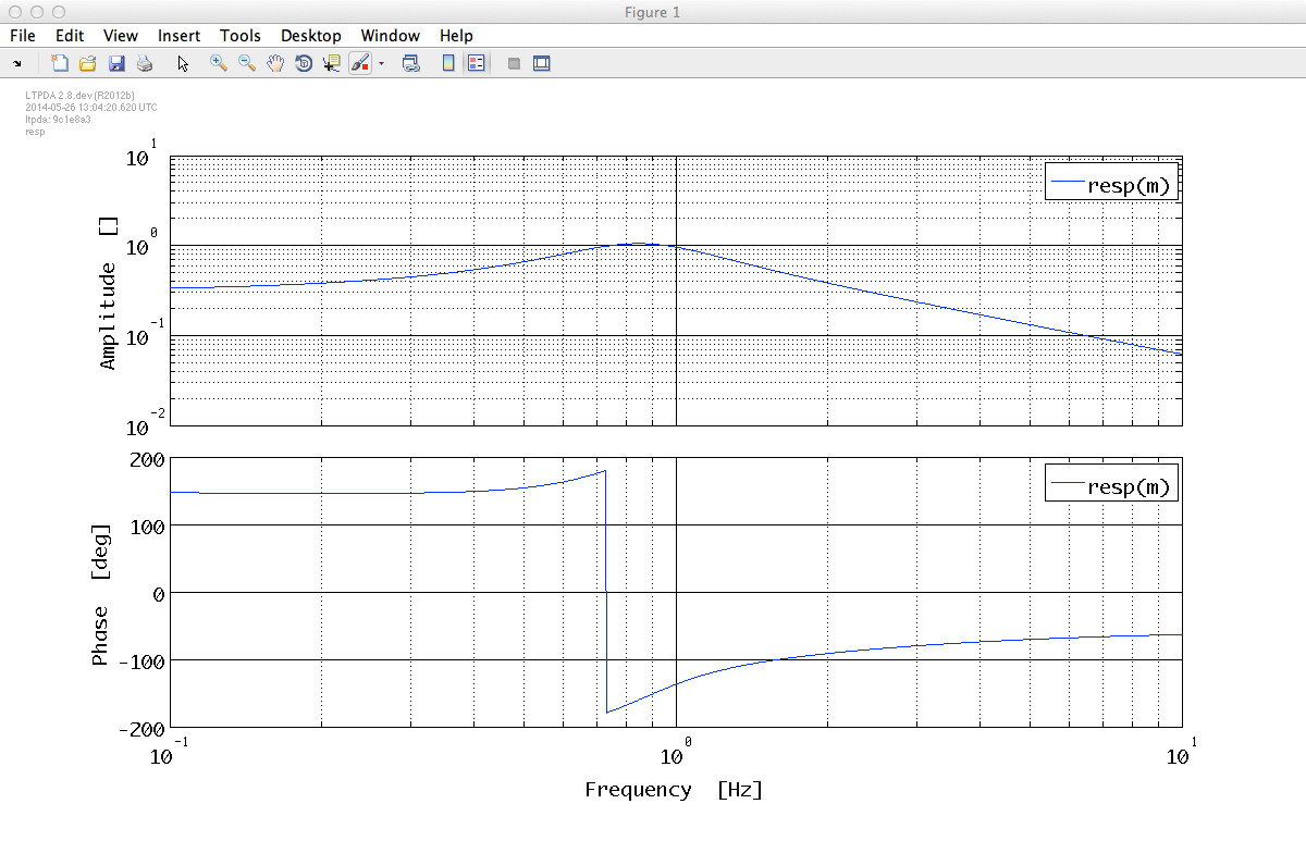
We can now take a look at the response of the transfer function that we have just created. We can specify the frequency region in what we are interested with the plist of the resp function. For example, we would like to evaluate our transfer function model from f1 = 0.1 Hz to f2 = 10 Hz.

resp(m, plist('f1', 0.1, 'f2', 10))

$Response of a parfrac model$

Pole zero model representation

Rational representation