

| LTPDA Toolbox™ | contents | |
In this section we give an overview of the main elements we will use in the following to simulate some experiments in the LTP and estimate system parameters from them. In order to capture the main concepts of the analysis we perform a limited analysis based on the following constraints:
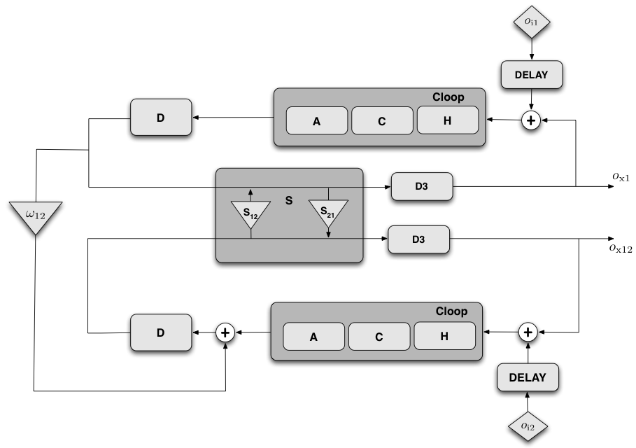
The scheme above show the main elements in the model: D stands for the dynamics of the test mass; S is the sensor (interferometer in our case); the control is split in the controller transfer functions (H), the decoupling matrix (C) and the actuators (H). DELAY and D3 are delay boxes that we will not use in our exercise. In the exercise we will use two ssm models implementing the previous scheme: one to generate the data (which) include noise sources and a second used for parameter estimation (where we do not need the noise inputs). These are the following:
| Model name | Comment |
|---|---|
|
LTP |
noise sources not included (type: help ssm_model_LTP) |
|
LPF |
noise sources included (type: help ssm_model_LPF) |
The parameters relevant for our analysis are described in the table below. The names are according to the notation in the ssm models
| Parameter | Description |
|---|---|
|
FEEPS_XX |
FEEPs actuation gain in X direction |
|
CAPACT_TM2_XX |
Capacitive actuation in TM2 in X direction |
|
IFO_X12X1 |
Interferometer cross-coupling X1 -> X12 |
|
EOM_TM1_STIFF_XX |
TM1 stifness in X direction (squared) |
|
EOM_TM2_STIFF_XX |
TM2 stifness in X direction (squared) |
We will apply two signals to the system. These follow the prescription described in the technical note S2-UTN-TN-3045. Since these are quite used, the LTPDA contains two built-in models to create them in a single line. The first experiment will inject a sinusoid sequence to the x1 channel and the second experiment will inject a different sinusoid sequence to the x12 channel. Hence, the experiments we will study can be summarized in the following table:
| Experiment name | Signal applied | Injection port |
|---|---|---|
|
Inv0001 |
built-in model: 'signals_3045_1_1' |
GUIDANCE.IFO_x1 |
|
Inv0002 |
built-in model: 'signals_3045_1_2' |
GUIDANCE.IFO_x12 |
In this simplified analysis, our analysis of the displacement (or acceleration) measured on the test masses will only come from the X component of optical read-out for the two channels, x1 and x12. Hence, discarding the remaining degrees of freedom. We will add two quantities that will, as described in Topic 3, will be useful when translating displacement into acceleration noise. The summary of measured quantities (for each experiment) used in the analysis is the following:
| Output port | Description |
|---|---|
|
DELAY_IFO.x1 |
Interferometer x1 measurement |
|
DELAY_IFO.x12 |
Interferometer x12 measurement |
|
DFACS.sc_x |
Commanded force on spacecraft |
|
DFACS.tm2_x |
commanded force on test mass #2 |
| |
Introduction to LTPDA's parameter estimation tools | Create simulated experiment data sets | |
©LTP Team