

| LTPDA Toolbox™ | contents | |
In this section of the exercise we show how to creat
simulated experiment data sets.
First of all, we set a reference time for our
experiment. The t0 can be defined as follows.
     clear all
     % Define a reference time for the experiments
     t0 = time('2012-01-17 17:04:11.529 UTC');
The two experiments are in fact two separate injections of frequency sweeps in the first and the differential channel. This means that we create a signal of sinusoidals and a signal of zeros for each experiment. These injections are already built-in and can be constructed with the equivalent input key of a plist.
        %%% First channel (x1)

        % Create input signal from built-in model
        i1_1 = ao(plist('built-in', 'signals_3045_1_1'));

        % Adding reference time
        i1_1.setT0(t0);
We can call the zeropad function and add some zeros before and after the actual signal. These chuncks will be used to extract the simulated noise of the LTP system. The 'N' key of the plist defines the number of samples and with the 'position' key ('pre' or 'post') we can define where to add the zeros; before of after the built-in signal constructed.
        % Add zeros before and after
        i1_1.zeropad(plist('N', 200000, 'position', 'pre'));
        i1_1.zeropad(plist('N', 20000, 'position', 'post'));

        % Set Name
        i1_1.setName('Inv0001_x1_inj');
The input of zeros to inject to the differential channel is easier to obtain. We construct an ao object with an input plist. The 'Yvals' would be all zeros and the number of samples the same as inj_1_1.
    %%% Second channel (x12)

    % Input signal for second channel is zero
    % We build this signal by forcing it to lay on the same time values as the i1_1
    i1_2 = ao(plist('Yvals', zeros(size(i1_1.x)), 'fs', 10, 't0', t0, 'Yunits', 'm'));
    i1_2.setToffset(i1_1.toffset);
    i1_2.setName('Inv0001_x12_inj');
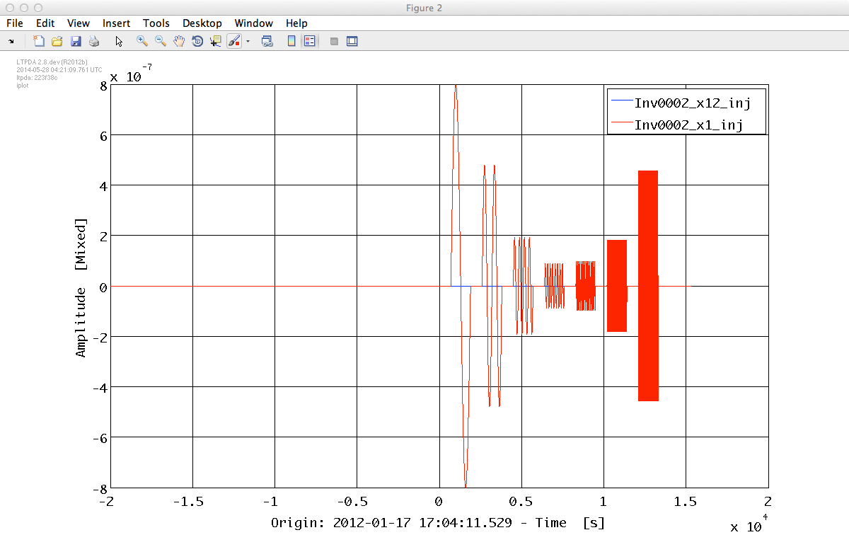
Plotting the injection for the two channels in the first experiment produces the figure below.
 % Plot injection signals
        iplot(i1_1, i1_2)

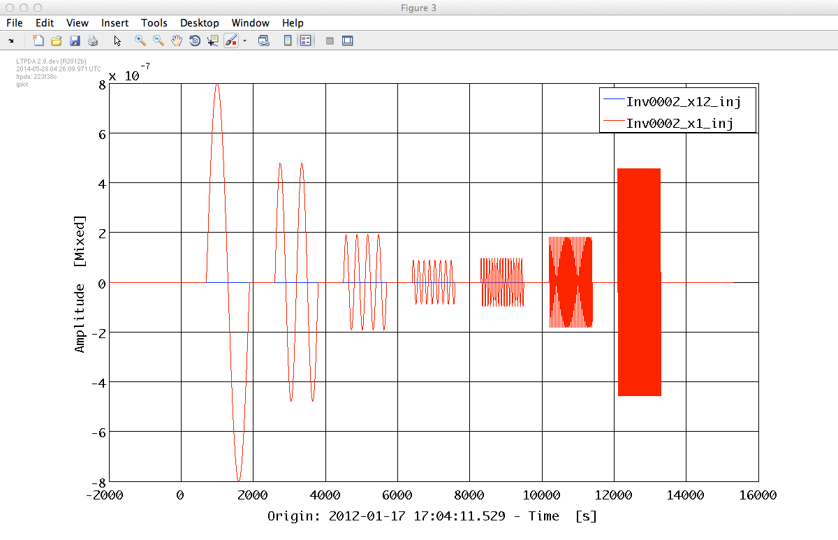
The same would apply for the second experiment with the exception that:
     %% Generate data for experiments Inv0002

     %%% Second channel

     i2_2 = ao(plist('built-in','signals_3045_1_2'));
     i2_2.setT0(t0);
     i2_2.zeropad(plist('N', 200000,'position', 'pre'));
     i2_2.zeropad(plist('N', 20000,'position', 'post'));
     i2_2.setName('Inv0002_x1_inj');

     %%% First channel

     i2_1 = ao(plist('Yvals', zeros(size(i2_2.x)), 'fs', 10, 't0', t0));
     i2_1.setToffset(i2_2.toffset);
     i2_1.setName('Inv0002_x12_inj');

     iplot(i2_1, i2_2)
To generate our data sets we will use the built-in model LPF which assemble in a single object all the subsystems together with a default profile of noise inputs. For more information on the model type
help ssm_model_LPF
We will build this model at the same time that we set some parameters to a certain numerical value. These are the parameters that we will be estimating in later in this exercise and are described in the following table
| Key | Value | Description |
|---|---|---|
|
'FEEPS_XX' |
0.82 |
FEEPs actuation gain in X direction |
|
'CAPACT_TM2_XX' |
1.08 |
Capacitive actuation in TM2 in X direction |
|
'IFO_X12X1' |
0.0004 |
Interferometer cross-coupling X1 -> X12 |
|
'EOM_TM1_STIFF_XX' |
1.3e-6 |
TM1 stifness in X direction (squared) |
|
'EOM_TM2_STIFF_XX' |
1.9e-6 |
TM2 stifness in X direction (squared) |
On our implementation, we first define a string params with the name of the parameters, an array values with the numerical values previously defined and then we input them to the plist that defines our model.
      % Define parameters and nominal values
      params = {...
            'FEEPS_XX', ...         % Coupling of the commanded force along X to the applied force along X
            'CAPACT_TM2_XX', ...    % Actuaction cross-coupling of TM2 force along X to TM2 force along X
            'IFO_X12X1', ...        % The coupling of the x position of TM1 to the estimated x position of TM2 w.r.t. TM1
            'EOM_TM1_STIFF_XX', ... % Total stiffness of TM1 along X when moving along X.
            'EOM_TM2_STIFF_XX' ...  % Total stiffness of TM2 along X when moving along X.
            };
      values = [0.82 1.08 0.0004 1.3e-6 1.9e-6];

      % Create plist defining how we want to build the model
      simPlist = plist('built-in','LPF', ... % From built-in models
                       'DIM', 1, ...                        % We use a one dimensional model
                       'CONTINUOUS', false, ...             % The model descrete
                       'param names', params, ...           % Parameter names
                       'param values', values, ...          % Parameter values
                       'VERSION', 'Best Case June 2011'); % Version of the LPF

      % Create the LPF model.
      LPF = ssm(simPlist);

      %% save model
      save(LPF, 'generation_LPF_model.mat');
To produce a set of data we first need to define how the different noise sources are correlated, i.e. the noise covariance. The ssm class provides a method that provides this information (although the user is free to provide his own covariance matrix)
        %% Generate noise covariance for experiments 1 & 2
        cov = LPF.generateCovariance;
Next, define the ports where the inputs are injected abd where the outputs are measured
        % Define input and output channels
        inNames = {...
              'GUIDANCE.IFO_x1'  ...   % x1 control coordinate, read by o1 IFO
              'GUIDANCE.IFO_x12' ...   % x12 control coordinate, read by differential IFO
              };

        outNames = {...
              'DELAY_IFO.x1'  ...      % o1 IFO
              'DELAY_IFO.x12' ...      % o12 IFO
              'DFACS.sc_x'    ...      % commanded force on SC
              'DFACS.tm2_x'   ...      % commanded force on TM2
              };
And add this information in a plist and use it to call the method simulate
    pl_sim_Inv0001 = plist(...
                'aos variable names', inNames(1),...
                'aos', i1_1,...
                'return outputs', outNames,...
                'cpsd variable names', cov.find('names'), ...
                'cpsd', cov.find('cov'), ...
                'displayTime', true,...
                't0', t0);

    % Inv0001: run the simulation
    % In this investigation, the guidance is applied on the x1 control coordinate, read by o1 IFO
    pl_sim_Inv0001 = plist(...
                        'aos variable names', inNames(1),...       % Names of the inputs
                        'aos', i1_1,...                            % injection signals
                        'return outputs', outNames,...             % Names of the outputs
                        'cpsd variable names', cov.find('names'), ...
                        'cpsd', cov.find('cov'), ...
                        'displayTime', true,...
                        't0', t0);

    % Generate data
    o_0001 = LPF.simulate(pl_sim_Inv0001);
We unpack to recover all the different output ports we ask for in the plist
       % The output Analysis Objects are grouped in a matrix object, so we need to index them
       [o1_0001, o12_0001, Fsc_0001, Ftm2_0001] =  o_0001.unpack;
And repeat the same operation to produce the data set for the second experiment. Notice that in the plist we change the input port (in order to inject the signal in the differential channel) and the injected signal is now i2_2
        % Inv0002: run the simulation
        % In this investigation, the guidance is applied on the x12 control coordinate, read by differential IFO
        pl_sim_Inv0002 = plist(...
                      'aos variable names', inNames(2), ...
                      'aos', i2_2, ...
                      'return outputs', outNames, ...
                      'cpsd variable names', cov.find('names'), ...
                      'cpsd', cov.find('cov'), ...
                      'displayTime', true, ...
                      't0', t0);

        % Generate data
        o_0002 = LPF.simulate(pl_sim_Inv0002);

        % The output Analysis Objects are grouped in a matrix object, so we need to unpack them
        [o1_0002, o12_0002, Fsc_0002, Ftm2_0002] =  o_0002.unpack;
The methods that we will use in the analysis work, for simplicity, with matrix objects. These objects allow to put several time series together to refelct the fact that our analysis requires many channels. In this particular case only two: x1 and x12. The objects are built as follows:
    %% Build matrix objects

    % Group the guidance injection signals of both experiments in the same matrix model
    inj_signal(1) = matrix(i1_1, i1_2, plist('shape', [2 1]));
    inj_signal(2) = matrix(i2_1, i2_2, plist('shape', [2 1]));

    % Group the measured outputs of both experiments in the same matrix model
    meas_signal(1) = matrix(o1_0001, o12_0001, plist('shape', [2 1]));
    meas_signal(2) = matrix(o1_0002, o12_0002, plist('shape', [2 1]));

    % Group the commanded forces of both experiments in the same matrix model
    cmd_forces(1) = matrix(Fsc_0001, Ftm2_0001, plist('shape', [2 1]));
    cmd_forces(2) = matrix(Fsc_0002, Ftm2_0002, plist('shape', [2 1]));
Once these objects are built, we can easily split our original data into the different segments of interest: we take a short segment where the input was applied for the in and out object, and a long segment without injected signal for the noise.
    % Split in times to get input, output, noise and commanded forces chunks
    in    = split(inj_signal, plist('times', [-2000 inf]));
    out   = split(meas_signal, plist('times', [-2000 inf]));
    noise = split(meas_signal, plist('times', [-inf -2000]));
    Fcmd  = split(cmd_forces, plist('times', [-inf -2000]));
Each of these contains two matrix objects (one for each experiment), with two time series (for x1 and x12) within. We can take a look at the objects for the second experiment:
    % Plot injected signal in 2nd experiment
    in(2).iplot
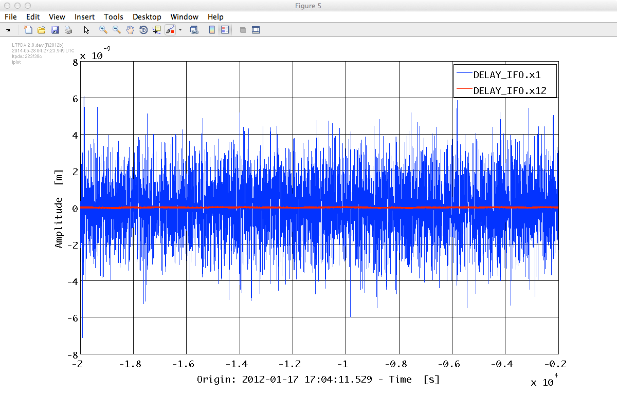
    % Plot measured signal in 2nd experiment
    out(2).iplot

    % Plot initial noise segment in 2nd experiment
    noise(2).iplot
    % Plot commanded forces in 2nd experiment
    Fcmd(2).iplot

Finally, we just need to save the objects we have just created. We will use them later for parameter estimation.
        %% save objects

        save([o_0001 o_0002], 'full_signal.mat');
        save(inj_signal, 'inj_signal.mat');
        save(in, 'input.mat');
        save(out, 'output.mat');
        save(noise, 'noise.mat');
        save(Fcmd, 'cmdForces.mat');
| |
A simplified LPF system identification experiment | Build state-space LTP models for system identification | |
©LTP Team