LTPDA Toolbox™

contents

Introduction to LTPDA's parameter estimation tools

In this topic we will rum some parameter estimation analysis on LTP simulated data. Although the analysis will run on ssm objects, the basics of the analysis and tools used can be understood in the following terms. Assume a system described (in frequency domain) as follows,

where we have an applied input (s) that goes through a system defined by a set of transfer functions (G) to produce a measured output (o), that is usually contaminated by a random process (n). Notice that in our exercise we use two LTP measurement, x1 and x12 and, therefore in reality we will be dealing with a 2D problem. Our system decomposed in components (and omitting dependences) is:

Our aim is to obtain the parameters via the dependence on the transfer function. We will use two different methods for that.

Linear Parameter Estimation with Singular Value Decomposition

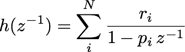
The first approach is based on least-squares. If we expand the transfer function and keep it to the first order,

If we do not consider 2nd order terms, we get a constant zeroth order term and the parameters enter only with a linear dependence. This equation define a linear system that can be solved analytical.

Whitening filter

It is worth mentioning that to correctly apply the least-squares approach, the noise must be uncorrelated and therefore the method will need to whiten (or uncorrelate) the data. In a 1D case, the process requires to fit the square root of the noise power spectrum density with a digital filter

and use the inverse of that filter to 'whiten' the data. In 2D systems, like the ones treated here the procedure is more involved, implying the eigendecomposition of the cross-power spectrum matrix.

Implementation

In LTPDA, the previous scheme is implemented in different methods that the user can tune and apply. In particular, for this analysis we will use a method to fit a frequency domain object

     % Fit frequency domain (continuous)
      out = sDomainFit(in, pl_fit);
     % Fit frequency domain (discrete)
      out = zDomainFit(in, pl_fit);

A method that builds the whitening filters

     % Build whitening filter
     out = buildWhitener1D(in, plw);

An the method to solve the linear system and get the parameters

     % Run Linear Fit
     params = linfitsvd(in, plist);

Markov Chain Monte Carlo

The second apporoach that we will use is a statistical method based on a random sampling of the parameter space. In this method, new samples are generated using a Markov Chain mechanism and in each jump (or step) in the parameter space, the likelihood is calculated. According to our previous description, the likelihood reads as

where the C stands here for the covariance matrix between channels, that we build computing the cross-power spectrum matrix. This term plays the role here of the whitening filter in the previous method. The MCMC will sample the parameter space looking for the parameters that maximize the likelihood, eventually reaching the maximum likelihood estimates. Since the method will draw random samples during this process, we will be able to trace the shape of the likelihood surface during the process from where we will be able to derive the posterior probability distribution of the parameters.

Fisher matrix

An important tool in this section will be the Fisher matrix, usually defined as

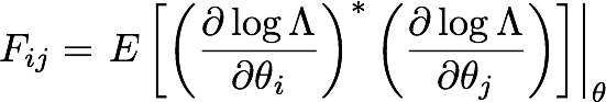
which can be used to derive a lower bound for the variance of an unbiased estimator. This result is known as the Cramer-Rao bound,

We will use this in two different steps. First, to get an estimate of the expected errors that we should get for each parameter (and correlations between them). In this sense, the Fisher matrix is directly related with the design of our experiment. Second,we will use the inverse of the Fisher matrix as an input to the MCMC. It is a standard procedure in MCMC algorithms to use a proposal distribution which encodes the information of this covariance matrix to draw new samples in the Markov Chain process. In that way we increase efficiency by 'jumping' into the right directions. In our case the proposal distribution will be a multivariate gaussian with the covariance given by the inverse of the Fisher matrix

Implementation

Methods to implement this analysis scheme are, first, the one to compute the inverse of the Fisher matrix

     % Compute inverse of Fisher matrix
     out = crb(in, pl_crb);

An one implementin the MCMC

     % Run MCMC
     out = mcmc(in, pl_mcmc);

References

• F Ferraioli et al., Calibrating spectral estimation for the LISA Technology Package with multichannel synthetic noise generation, Phys. Rev. D 82, 042001 (2010).
• M Nofrarias et al., Bayesian parameter estimation in the second LISA Pathfinder mock data challenge, Phys. Rev. D 82, 042001 (2010).
• F Ferraioli et al., Quantitative analysis of LISA pathfinder test-mass noise, Phys. Rev. D 84, 122003 (2011).
• M Nofrarias et al., Parameter estimation in LISA Pathfinder operational exercises arXiv: gr-qc:1111.4916 (2011).

Topic 5 - Introduction to system identification of LPF.

A simplified LPF system identification experiment

©LTP Team