LTPDA Toolbox™

Simulating LPF noise

Here we will simulate the LPF system using the internal noise generator. In Topic 4 you will see how to inject signals into the simulation.

LPF noise simulations: single noise source

You can set up the simulation to simulate a single noise source for LPF by specifying a single input name and a value for the variance of that noise. Let's suppose we want to simulate the effect of interferometer readout noise on the X1 interferometer and look how that appears in the two longitudinal interferometer outputs. Here's how to do it:

      % Build the default version of the LPF model      
      lpf = ssm(plist('built-in', 'LPF'));
      
      % Define the simulation plist for a 10000 sample simulation      
      simPlist = plist(...
                  'CPSD Variable Names', 'DIST_IFO_READOUT_NOISE.x1', ...
                  'CPSD', 1, ...
                  'Return outputs', {'IFO.x1', 'IFO.x12', 'DIST_IFO_READOUT.x1'}, ...
                  'Nsamples', 10000 ...
                  );
                  
      % Run the simulation      
      out = simulate(lpf, simPlist);

The output of the ssm/simulate method is a matrix object containing a series of time-series analysis objects, one for each requested output. Please notice that we requested as output also the quantity 'DIST_IFO_READOUT.x1' which is an (internal) input to the system, but can also be passed in output.
You can plot the two time-series by doing:

      % Plot on subplots       
      iplot(out, plist('arrangement', 'subplots'));
      
      % Or, unpack them and plot individually      
      [o1, o12, noise] = unpack(out);
      iplot(o1)
      iplot(o12)
      iplot(noise)

It's also interesting to look at the spectra of these two outputs. Since we do not plan to combine the spectra later on, we delegate to the spectral estimator ao/psd the calculation of the square root of the spectra themselves, so to ease the plotting steps. Here's how:

      % Plist for configuring the PSD estimator      
      psdPlist = plist(...
                  'navs', 16, ...
                  'scale', 'ASD', ...
                  'order', 1, ...
                  'win', 'BH92' ...
                  );
      
      % Estimate the PSD of each output      
      [S_o1, S_o12, S_noise] = psd(o1, o12, noise, psdPlist);
            
      % Plot the results      
      iplot(S_o1, S_o12, S_noise);
      
      % Note: you can also use the matrix/psd method      
      S_out = psd(out, psdPlist);
      
      % Unpack them and plot individually      
      [S_o1, S_o12, S_noise] = unpack(S_out);
      iplot(S_o1, S_noise)
      iplot(S_o12)

Covariance or CPSD?

The ssm/simulate method has two possible noise configuration inputs. Both use the internal noise generator. The difference is simply in the scaling:

When specifying the 'CPSD', the noise is scaled according to the sample rate of the simulation so to preserve the signal energy content.
When specifying the 'COV', the scaling is not performed.

As such, most of the time you will want to use the 'CPSD' inputs.

LPF noise simulations: two correlated noise sources

Simulating with more than one noise source requires setting of the inputs and (co-)variance just as in the single noise case. Suppose we want to activate the readout noise in both the X1 and X12 IFO. And further suppose that these two readout noises should be correlated. To simulate this, we should do:

      
      % Define the simulation plist for a 100000 sample simulation      
      simPlist = plist(...
                  'CPSD Variable Names', {'DIST_IFO_READOUT_NOISE.x1', 'DIST_IFO_READOUT_NOISE.x12'}, ...
                  'CPSD', [1 0.5; 0.5 1], ...
                  'Return outputs', {'IFO.x1', 'IFO.x12', 'DIST_IFO_READOUT.x1', 'DIST_IFO_READOUT.x12'}, ...
                  'Nsamples', 100000 ...
                  );
                  
      % Run the simulation      
      out = simulate(lpf, simPlist);

We can now extract the outputs and look at their spectra and cross-spectra, as well as the coherence between the measured X1 and X12 signals:

      
      % Unpack the signals from the simulation output matrix      
      [o1, o12, x1noise, x12noise] = unpack(out);
                                    
      % Estimate PSD of the measured outputs      
      [S_o1, S_o12] = psd(o1, o12, psdPlist);
      
      % Estimate CPSD of the measured outputs      
      S_o1o12 = cpsd(o1, o12, psdPlist);

      % Estimate COHERENCE of the measured outputs      
      C_o1o12 = cohere(o1, o12, psdPlist);
      
      % Plot results      
      iplot(S_o1, S_o12, abs(sqrt(S_o1o12)));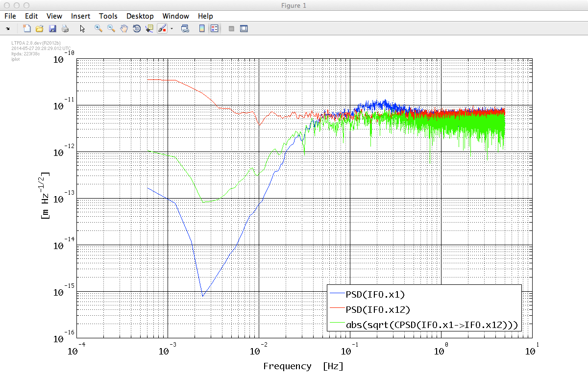

The warnings shown on the terminal are associated with the parameters that are peculiar only to the ao/psd method, and are not recognized by the other spectral estimators. We can ignore them, and take advantage of re-using the plist for the common parameters (window, number of averages, detrending order). This should result in a plot something like the one below:

LPF noise simulations: all noise sources on

Simulating with all the noise sources on works just the same as the above examples. However, there are 95 noise inputs to the LPF model and specifying each of them would be quite painful. So, we have a shortcut for doing this. There is an ssm method called generateCovariance which creates a suitable covariance matrix for you as well as a list of the all the noise input port names. The covariance matrix it generates is diagonal and as such all input noises are specified as uncorrelated. To use this method in conjunction with ssm/simulate you can follow the example. The covariance matrix is included in a plist object, together with other informations, and as such it must be extracted from the plist to be passed as a numeric parameter.

      
      % Create a covariance matrix and port list sized for our LPF model      
      cov_matrix = lpf.generateCovariance();
                                    
      % Define the simulation plist for a 100000 sample simulation      
      simPlist = plist(...
                  'CPSD Variable Names', cov_matrix.find('names'), ...
                  'CPSD', cov_matrix.find('cov'), ...
                  'Return outputs', {'IFO.x1', 'IFO.x12', 'DFACS.sc_x', 'DFACS.tm2_x'}, ...
                  'Nsamples', 100000 ...
                  );
                  
      % Run the simulation      
      out = simulate(lpf, simPlist);

In this case, we are asking to report at the output the reading of the X1 IFO, as well as the forces that the DFACS controller calculates and commands to the FEEPs, so to control the spacecraft along x, and to the FEE connected to the EH of the TM2, so to control TM2 itself along x.
We can look at the time-series and spectra in the usual way:

      
      % Unpack the signals from the simulation output matrix      
      [o1, o12, F_cmd_X, F_cmd_x2] = unpack(out);
                                    
      % Plot the IFO outputs and commanded forces along x      
      iplot(o1, o12);
      iplot(F_cmd_X, F_cmd_x2);
      
      % Estimate PSD of the measured outputs      
      [S_o1, S_o12, S_F_cmd_X, S_F_cmd_x2] = psd(o1, o12, F_cmd_X, F_cmd_x2, psdPlist);
      
      % Plot results      
      iplot(S_o1, S_o12);
      iplot(S_F_cmd_X, S_F_cmd_x2);

Simulating capacitive actuation noise

Changing system parameters