LTPDA Toolbox™

Changing system parameters

The statespace models in LTPDA have two types of parameters: configuration parameters, like 'DIM', 'VERSION', which are common to all ssm models, and system parameters which are model specific. These system parameters represent symbolic entries in the underlying statespace matrices. By default, when you build a ssm object, the system parameters are replaced by their numerical values and the model is returned in a fully numeric state. The numerical values that were substituted are stored in the 'numparams' field of the object. This field is a plist where each key represents the parameter name, and the corresponding value is the parameter value.

For example, suppose we build the LTP model like this:

      % Build the default version of the LTP model      
      ltp = ssm(plist('built-in', 'LTP'));

Then firstly you will see that the model is numeric:

      % Check if the model is numeric      
      ltp.isnumerical

We can inspect the numerical parameters that were substituted during the building process by looking at the field 'numparams' (numerical parameters):

      % List the numerical parameters      
      ltp.numparams

As you can see, the model has many parameters (351). A more useful way to view them is:

      % View the 'numparams' plist in MATLAB's documentation browser      
      ltp.numparams.tohtml

Since this field is a plist, if you know the name of a parameter, you can search for its value like this:

      % Get the TM1 stiffness along x      
      w1 = ltp.numparams.find('EOM_TM1_STIFF_XX');

Hint: if you don't know the name of the parameter, you can search using the plist/regexp method. For example:

      % Search for all stiffness values      
      subsetPlist = ltp.numparams.regexp('stiffness');

You can even chain these searches together:

      % Search for all stiffness values      
      subsetPlist = ltp.numparams.regexp('stiffness').regexp('TM1');

Setting system parameters at build time

You can override the default system parameters at build time by specifying the parameter name and a value in the configuration plist used for building the model. For example, let's set the stiffness of TM1 to a different value when building our LTP model:

      
      % Build the default version of the LTP model      
      modelPlist = plist(...
                      'built-in', 'LTP', ...
                      'EOM_TM1_STIFF_XX', 1e-6 ...
                      );
      
      % Build the LTP model with our configuration plist      
      ltp = ssm(modelPlist);

Note: In the current version of the LPF models, stiffness terms are specified as positive. This will likely change in future versions.

Confirm that your value for the stiffness was indeed used:

      % Get the TM1 stiffness along x      
      w1Used = ltp.numparams.find('EOM_TM1_STIFF_XX')

Creating symbolic models

The default is to build models completely numeric, but you can also build symbolic models. One limitation of doing this is that the model needs to be built continuous rather than discrete. This imposes further constraints on the models you are able to build, especially when it comes to the version of the DFACS model that you build because we don't have continuous versions of the DFACS for all versions.

To build the 'Standard' version of LTP continuous and with some symbolic parameters, you can do:

      
      % Build the default version of the LTP model      
      modelPlist = plist(...
                      'built-in', 'LTP', ...
                      'SYMBOLIC PARAMS', {'EOM_TM1_STIFF_XX', 'EOM_TM2_STIFF_XX'}, ...
                      'continuous', true ...
                      );
      
      % Build the symbolic LTP model with our configuration plist      
      ltp = ssm(modelPlist);

If you build the LTP model like this you will see, firstly, that it is not numeric, and secondly that it has a time-step of zero, i.e., it is continuous.

      
      % Check if the model is numeric      
      ltp.isnumerical
      
      % Check if the model is continuous      
      ltp.timestep

You can also see that the 'params' field contains two parameters, the ones you specified when constructing the model. Like the 'numparams' field, the 'params' field is also a plist.

      % List the symbolic parameters      
      ltp.params

Setting system parameters at run time

Once you have a symbolic model, you can change the values of those symbolic parameters by using the ssm/setParameters method. For example, let's set the two stiffness values we kept symbolic in the model we built above:

      
      % Set the values of the two stiffness parameters      
      ltp.setParameters('EOM_TM1_STIFF_XX', 1e-6, 'EOM_TM2_STIFF_XX', 3e-6);
            
      % Check the values were set      
      ltp.params
      
      % View the 'params' plist in MATLAB's documentation browser      
      ltp.params.tohtml

Note: by calling setParameters with no outputs, we modify our existing model. If we did give an output variable, then the original model would be copied, the parameters set on the copy, and then the copy returned, leaving the original model untouched.

Simulating with a symbolic model

Before we can simulate with this symbolic model, we have to make the model discrete. Before we can do that, we have to make the model numeric. Making the model numeric means substituting all symbolic parameters with their numeric values. To do that, we use the ssm/subsParameters method like this:

      
      % Substitute all symbolic parameters with their numeric values      
      numericLTP = ltp.subsParameters;
      
      % Confirm there are no symbolic parameters remaining      
      numericLTP.params

The model is now numeric but still continuous. We can already look at the response of the model in the frequency domain using ssm/bode. For example, we can look at the transfer function from differential force applied to the TMs to the differential displacement sensed by the IFO:

      % Define a plist for bode
      bodePlist = plist(...
                    'inputs', 'SIGNAL_TM12.x', ...
                    'outputs', 'DELAY_IFO.x1', ...
                    'f', logspace(-4, log10(0.5), 1000) ... % from 0.1mHz to 0.5Hz
                    );
      
      % Compute system response
      out = numericLTP.bode(bodePlist);
      
      % Plot response
      iplot(out);

Now we can go ahead and discretize the model using ssm/modifyTimeStep. On-board LPF the DFACS controllers are discretized at 10Hz, so we'll do the same here:

      
      % Modify the time-step of the model to 0.1s (10Hz)      
      dLTP = numericLTP.modifyTimeStep(0.1);
            
      % Confirm the model has this timestep
      dLTP.timestep

Again, we can compute the same bode response as above and explore the effect of discretizing the model:

      
      % Compute system response
      dout = dLTP.bode(bodePlist);
      
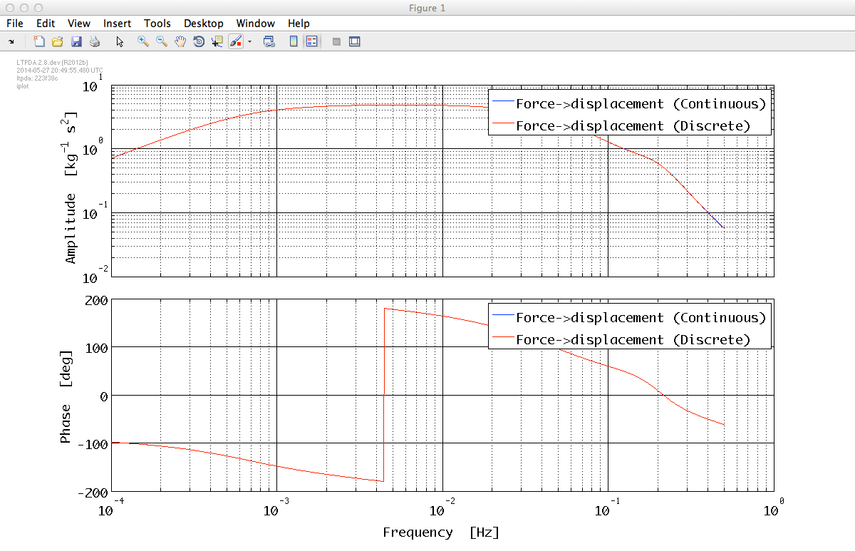
      % Get the continuous response and set its name
      contResp = out.unpack;
      contResp.setName('Force->displacement (Continuous)');
      
      % Get the discrete response and set its name
      discResp = dout.unpack;
      discResp.setName('Force->displacement (Discrete)');
      
      % Compare the two bode plots
      iplot(contResp, discResp)

Discretizing a model is not an exact mapping, and should be used with care. It is always better, where possible, to build a discrete model from the outset. When doing that, each submodel is built discrete before assembling. Doing it this way round means that each model is built continuous, then assembled, and the final full system is discretized.

Since the model is now numerical and discrete, we can simulate the noise of the system just as we did earlier.

Simulating LPF noise

Simulate LPF with matched stiffness