

| LTPDA Toolbox™ | contents | |
In this section we want to investigate how the DIST_* models behave, by simulating them. Let's begin with the DIST_CAPACT model, that provides the force/torque noise associated with the electrostatic actuation in the LPF TMs. We build the standard version of the system:
  % Build the default version of the GRS CAPactive ACTuation noise model
  GRScapactNoise = ssm(plist('built-in', 'DIST_CAPACT'));
  %% Get help on the GRS CAPactive ACTuation noise model
  help ssm_model_DIST_CAPACT
  %% Obtain more details about this model
  GRScapactNoise.viewDetails
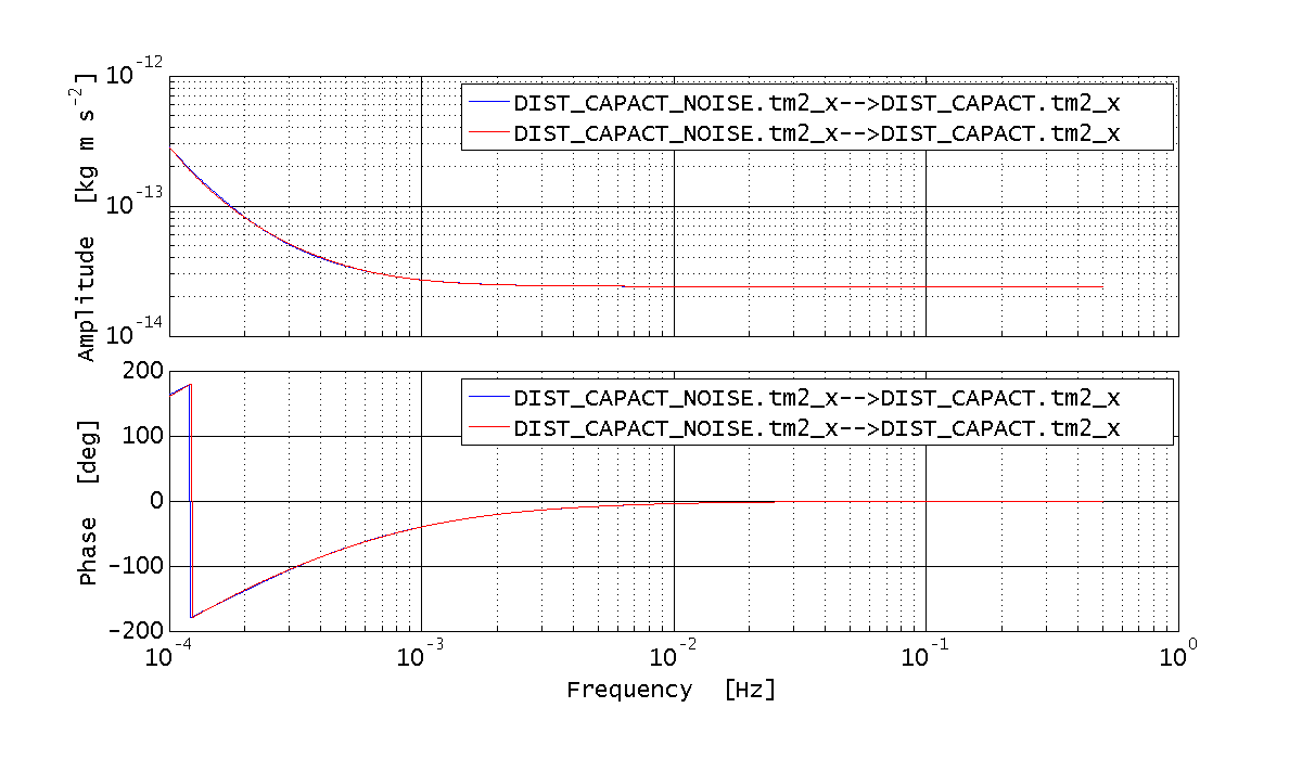
      %% Calculate the bode response of the noise coloring filter for the continuous system, tm2_x port
      tm2_xNoisePlist = plist(...
                          'inputs', 'DIST_CAPACT_NOISE.tm2_x', ...
                          'outputs', 'DIST_CAPACT.tm2_x', ...
                          'f', logspace(-4, log10(0.5), 1000) ... % from 0.1mHz to 0.5Hz
                          );

      bode_out                       = bode(GRScapactNoise, tm2_xNoisePlist);
      GRScapactNoise_tm2_x_cont_resp = bode_out.unpack();
| Remember: the output of bode is a matrix object. The single response we want (1 input to 1 output) is represented by the single ao inside the output matrix. So we unpack that single object from the matrix. |
In order to simulate the ssm models, we need to discretize them, by setting the time-step to a non-zero value.
  %% Discretize the system to be simulated at 1 Hz
  timestep = 1;
GRScapactNoise_discrete = GRScapactNoise.modifyTimeStep(timestep);%% Calculate the bode response of the noise coloring filter for the discrete system, tm2_x port bode_out = bode(GRScapactNoise_discrete, tm2_xNoisePlist); GRScapactNoise_tm2_x_disc_resp = bode_out.unpack(); %% Compare the transfer functions for the discrete and continuous case iplot(GRScapactNoise_tm2_x_cont_resp, GRScapactNoise_tm2_x_disc_resp);
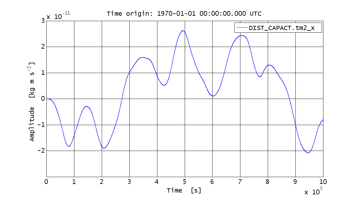
Let's assume we only want to simulate the effect of the force noise acting on TM2 along x, so we simulate a single noise source. We can do that by specifying a single input name and a value for the CPSD of that noise source:
  %% Simulate the system behavior: only tm2_x force noise
  % Simulation configuration plist
  simPlist_noise = plist(...
    'CPSD Variable Names', 'DIST_CAPACT_NOISE.tm2_x', ...
    'CPSD', 1, ...
    'Return outputs', {'DIST_CAPACT.tm2_x'}, ...
    'Nsamples', 1e6 ...
    );

  % Launch the simulation
  sim_output = GRScapactNoise_discrete.simulate(simPlist_noise);

  % Extract the AO with the force data
  out_tm2_x = sim_output.unpack();

  % Plot the results
  iplot(out_tm2_x)
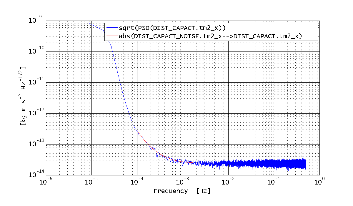
Eventually, we want to estimate the PSD of the force. We also want to compare the estimated PSD with the expected output of the coloring filter; in order to do that, we have to change the units, so to account for the fact that the input CPSD is expressed in Hz^-1.
  %% Estimate the PSD
  % PSD estimation configuration plist
  psdPlist = plist(...
    'scale', 'PSD', ...
    'order', 1, ...
    'win', 'BH92', ...
    'navs', 25 ...
    );

  % Estimate the PSD
  S_out_tm2_x = out_tm2_x.psd(psdPlist);

  % Plot the PSD and compare with the expected noise shape
  % We have to account for the unit of the input to the coloring filter
  GRScapactNoise_tm2_x_disc_resp.setYunits(sqrt(S_out_tm2_x.yunits));
  iplot(sqrt(S_out_tm2_x), abs(GRScapactNoise_tm2_x_disc_resp));
| |
Simulating harmonic oscillator noise | Simulating LPF noise | |
©LTP Team