

| LTPDA Toolbox™ | contents | |
Let's begin with a simple example, namely the harmonic oscillator. The system can be built easily, specifying the values for the key parameters (mass, spring constant, viscous damping coefficient):
  % Build a Harmonic Oscillator model
  % Physical parameters
  m     = .1;     % mass: 0.1 kg
  k     = 1e-2;   % spring constant: 1e-2 N / m
  vbeta = 1e-3;   % viscous damping coefficient: 1e-3 N s / m

  % Definition plist
  buildPlist = plist(...
              	'built-in', 'HARMONIC_OSC_1D', ...
                'm', m, ...
                'vbeta', vbeta, ...
                'k', k ...
                );

  % Build the ssm model
  harm_osc = ssm(buildPlist);
  %% Look at the model details
  harm_osc.viewDetails
%% Check if the model is continuous
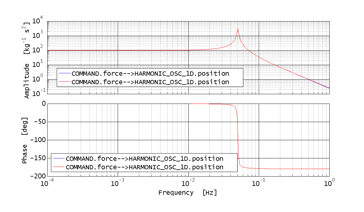
harm_osc.timestepNow we want to calculate the system transfer function of the input to the outputs, in order to estimate the effect of the sources. In order to do that, we can call the ssm/bode method, specifying the input port, the output port, and the frequency range. Here is an example, where we look at the response of the harmonic oscillator mass position to the application of an external force, in the range from 0.1 mHz t 1 Hz:
  %% Calcolate the bode response from force to displacement for the continuous system
  forceBodePlist = plist(...
    'inputs', 'COMMAND.force', ...
    'outputs', 'HARMONIC_OSC_1D.position', ...
    'f', logspace(-4, 0, 1000) ... % from 0.1mHz to 1Hz
    );

  bode_output              = bode(harm_osc, forceBodePlist);
  harm_osc_cont_resp_force = bode_output.unpack();
| NOTE: The output of bode is a matrix object. The single response we want (1 input to 1 output) is represented by the single ao inside the output matrix. So we unpack that single object from the matrix. |
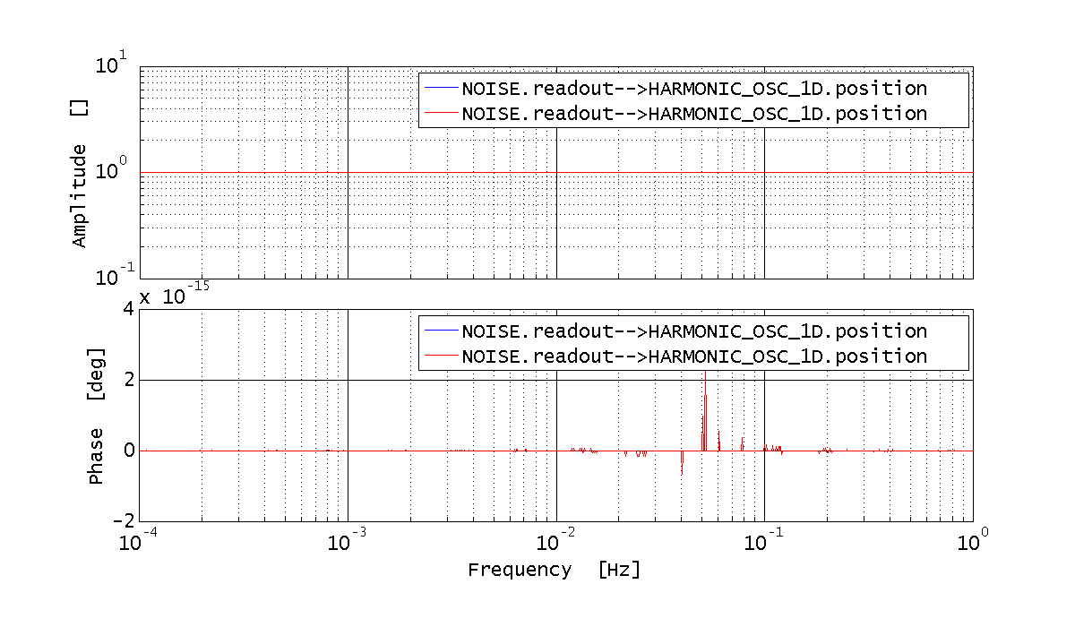
  %% Calcolate the bode response from readout noise to displacement for the continuous system
  readoutBodePlist = plist(...
    'inputs', 'NOISE.readout', ...
    'outputs', 'HARMONIC_OSC_1D.position', ...
    'f', logspace(-4, 0, 1000) ... % from 0.1mHz to 1Hz
    );

  bode_output                = bode(harm_osc, readoutBodePlist);
  harm_osc_cont_resp_readout = bode_output.unpack();
  %% Discretize the system to be simulated at 10 Hz
  timestep = 0.1;
  harm_osc_discrete = harm_osc.modifyTimeStep(timestep);
  % Calculate the bode response from force to displacement for the discrete system
  bode_output              = bode(harm_osc_discrete, forceBodePlist);
  harm_osc_disc_resp_force = bode_output.unpack();

  % Calculate the bode response from readout noise to displacement for the discrete system
  bode_output                = bode(harm_osc, readoutBodePlist);
  harm_osc_disc_resp_readout = bode_output.unpack();

  % Compare the transfer functions for the discrete and continuous case
  plot_plist = plist('linestyles', {'-', '--'});

  iplot(harm_osc_cont_resp_readout, harm_osc_disc_resp_readout, plot_plist);
  iplot(harm_osc_cont_resp_force, harm_osc_disc_resp_force, plot_plist);
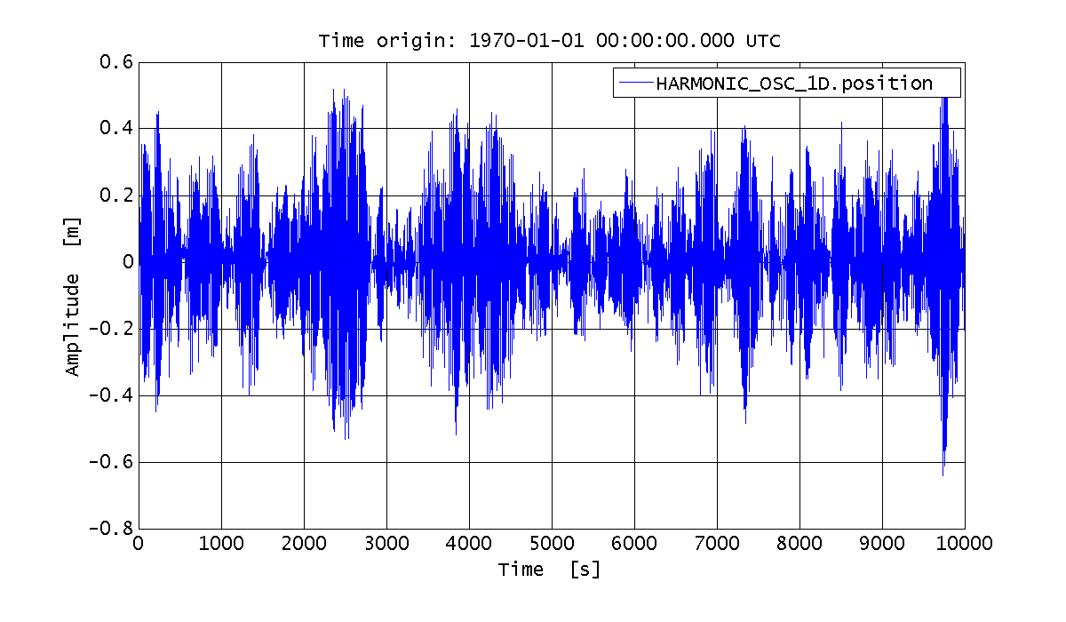
Let's assume we only want to simulate the effect of the external force noise, so we simulate a single noise source. We can do that by specifying a single input name and a value for the CPSD of that noise source:
  %% Simulate the system behavior: only force noise
  % Simulation configuration plist
  simPlist_force = plist(...
    'CPSD Variable Names', 'COMMAND.force', ...
    'CPSD', 1e-6, ...
    'Return outputs', {'HARMONIC_OSC_1D.position'}, ...
    'Nsamples', 100000 ...
    );

  % Launch the simulation
  sim_output = harm_osc_discrete.simulate(simPlist_force);

  % Extract the AO with the postion data
  out_force = sim_output.unpack();

  % Plot the results
  iplot(out_force)
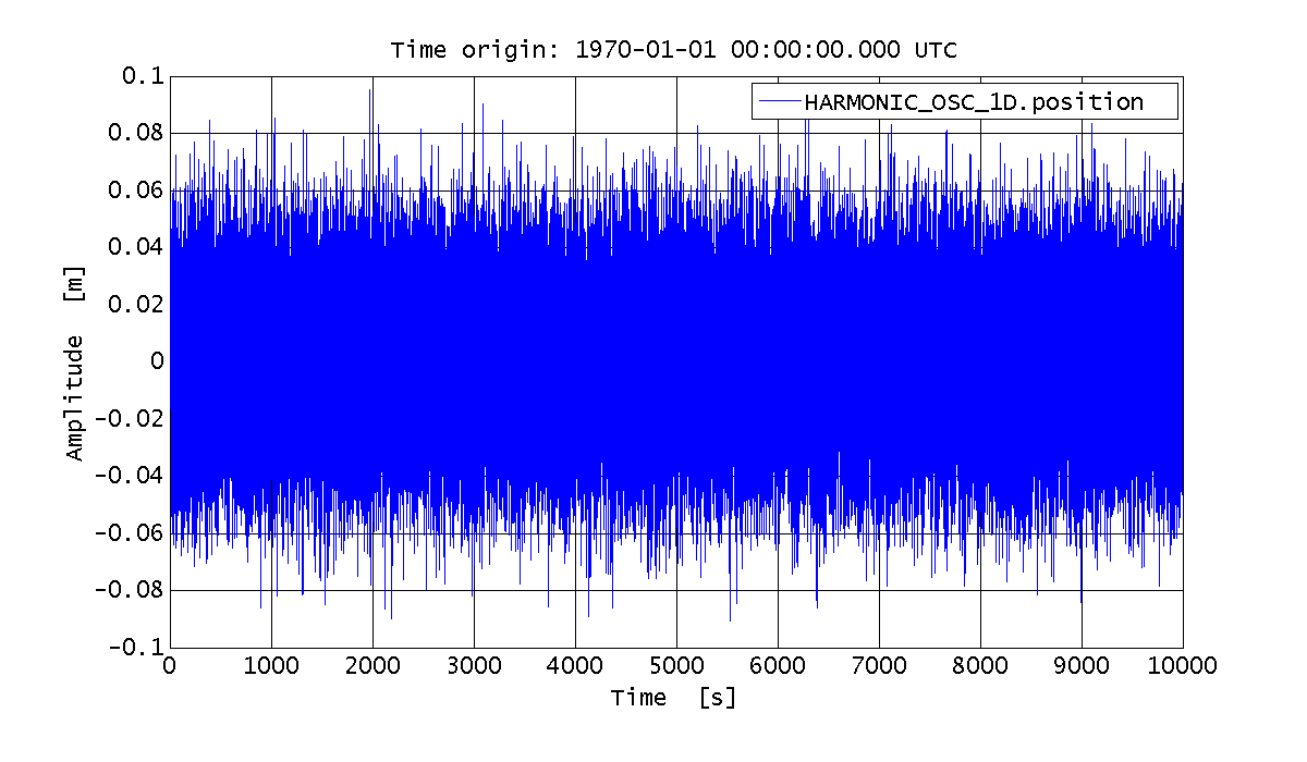
Similarly, let's assume we only want to simulate the effect of the readout noise, so we simulate a single noise source. We can do that by specifying a single input name and a value for the CPSD of that noise source:
  %% Simulate the system behavior: only readout noise
  % Simulation configuration plist
  simPlist_readout = plist(...
    'CPSD Variable Names', 'NOISE.readout', ...
    'CPSD', 0.01, ...
    'Return outputs', {'HARMONIC_OSC_1D.position'}, ...
    'Nsamples', 100000 ...
    );

  % Launch the simulation
  sim_output = harm_osc_discrete.simulate(simPlist_readout);

  % Extract the AO with the postion data
  out_readout = sim_output.unpack();

  % Plot the results
  iplot(out_readout)
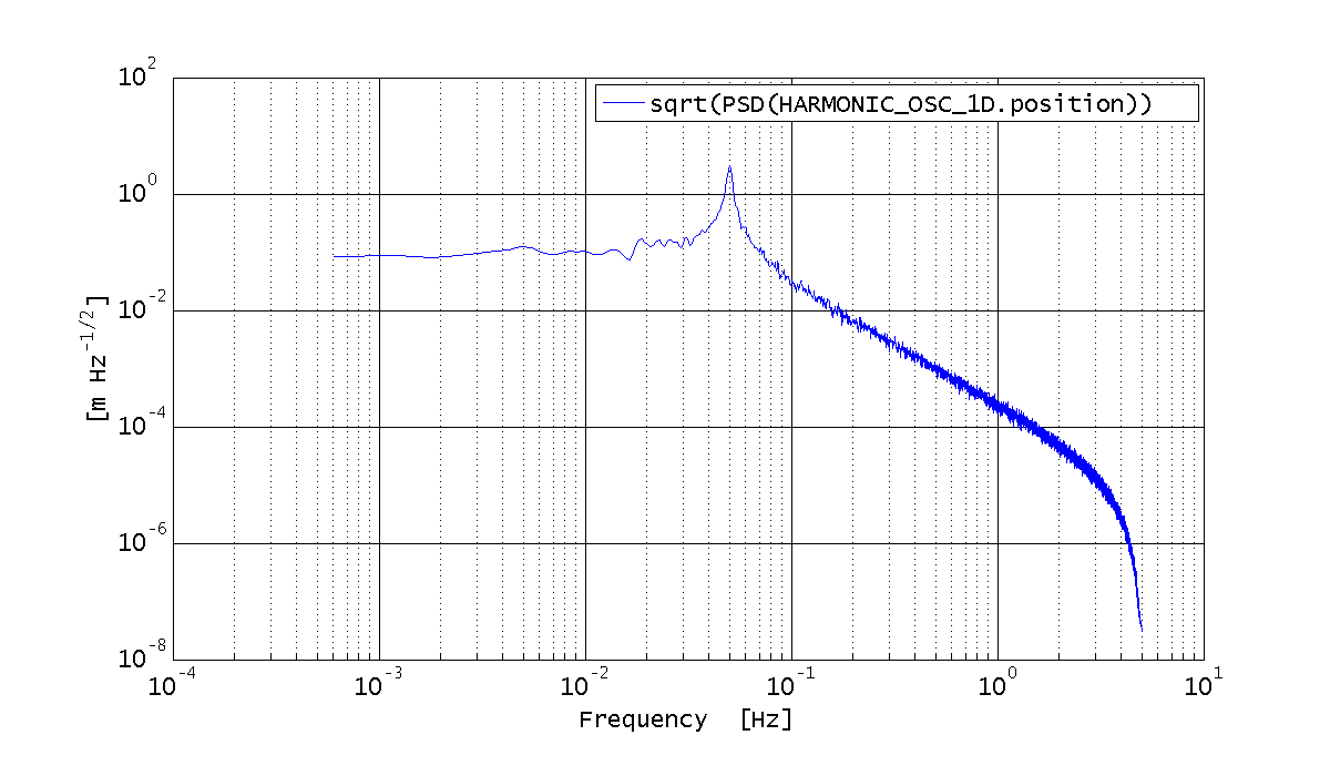
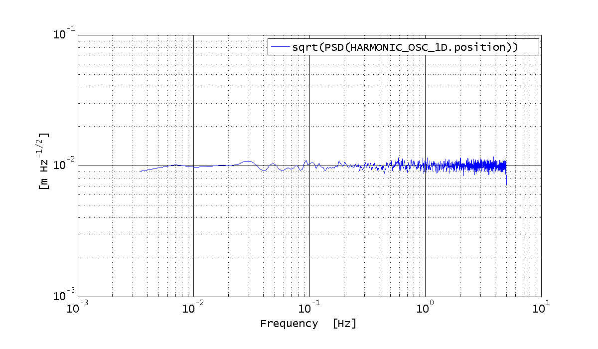
Eventually, we want to estimate the PSD of the displacement in the two cases. Just for curiosity, we change the number of averages in the two cases.
  %% Estimate the PSD
  % PSD estimation configuration plist
  psdPlist = plist(...
    'scale', 'PSD', ...
    'order', 1, ...
    'win', 'BH92' ...
    );

  % Estimate the PSD
  S_out_force   = out_force.psd(psdPlist.pset('navs', 16));
  S_out_readout = out_readout.psd(psdPlist.pset('navs', 100));

  % Plot the ASD (sqrt(PSD))
  iplot(sqrt(S_out_readout));
  iplot(sqrt(S_out_force));
| |
Simulating noise | Simulating capacitive actuation noise | |
©LTP Team