LTPDA Toolbox™

Noise whitening

Noise whitening in LTPDA

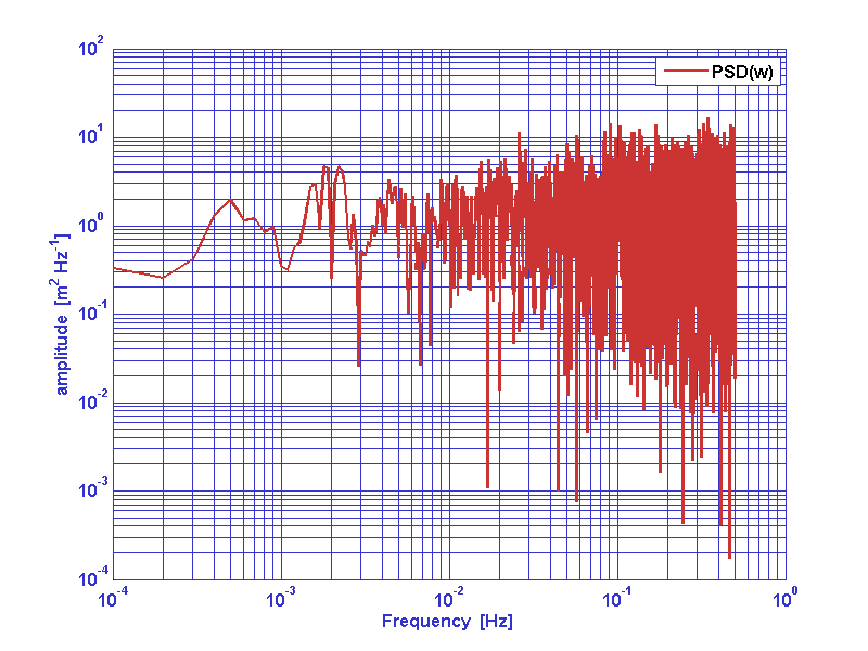
A random process w(t) is considered white if it is zero mean and uncorrelated:

As a consequence, the power spectral density of a white process is a constant at every frequency:

In other words, The power per unit of frequency associated to a white noise process is uniformly distributed on the whole available frequency range. An example is reported in figure 1.

**Figure 1:** Power spectral density (estimated with the welch method) of a gaussian unitary variance zero mean random process. The process *w(t)* is assumed to have physical units of `m` therefore its power spectral density has physical units of `m^2/Hz`. Note that the power spectral density average value is 2 instead of the expected 1 (unitary variance process) since we calculated one-sided power spectral density.

A non-white (colored) noise process is instead characterized by a given distribution of the power per unit of frequency along the available frequency bandwidth.
Whitening operation on a given non-white process corresponds to force such a process to satisfy the conditions described above for a white process.

In LTPDA there are different methods for noise whitening:

They accept time series analysis objects as an input and they output noise whitening filters or whitened time series analysis objects.

Whitening Algorithms

buildWhitener1D

buildWhitener1D performs a frequency domain identification of the system in order to extract the proper whitening filter. The function needs a model for the one-sided power spectral density of the given process. If no model is provided, the power spectral density of the process is calculated with the psd and bin_data algorithm.

The inverse of the square root of the model for the power spectral density is fit in z-domain in order to determine a whitening filter.
Unstable poles are removed by an all-pass stabilization procedure.
Whitening filter is provided at the output.

Whiten1D

whiten1D implements the same functionality of buildWhitener1D but it adds the filtering step so input data are filtered with the identified filter internally to the method.

Firwhiten

firwhiten whitens the input time-series by building an FIR whitening filter.

Make ASD of time-series.
Perform running median to get noise-floor estimate ao/smoother.
Invert noise-floor estimate.
Call mfir() on noise-floor estimate to produce whitening filter.
Filter data.

Whiten2D

whiten2D whitens cross-correlated time-series. Whitening filters are constructed by a fitting procedure to the models for the corss-spectral matrix provided. In order to work with whiten2D you must provide a model (frequency series analysis objects) for the cross-spectral density matrix of the process.

Whitening filters frequency response is calculated by the eigendecomposition of the cross-spectral matrix.
Calculated responses are fit in z-domain in order to identify corresponding autoregressive moving average filters.
Input time-series is filtered. The filtering process corresponds to:
w(1) = Filt11(a(1)) + Filt12(a(2))
w(2) = Filt21(a(1)) + Filt22(a(2))

Whitening noise in one-dimensional data

We can now test an example of the one-dimensinal whitening filters capabilities. With the following commands we can generate a colored noise data series for parameters description please refer to the ao, miir and filter documentation pages.

    
    fs = 1; % sampling frequency
    
    % Generate gaussian white noise
    pl = plist('tsfcn', 'randn(size(t))', ...
      'fs', fs, ...
      'nsecs', 1e5, ...
      'yunits', 'm');
    a = ao(pl);
    
    % Get a coloring filter
    pl = plist('type', 'bandpass', ...
      'fs', fs, ...
      'order', 3, ...
      'gain', 1, ...
      'fc', [0.03 0.1]);
    ft = miir(pl);
    
    % Coloring noise
    af = filter(a, ft);

Now we can try to white colored noise.

buildWhitener1D

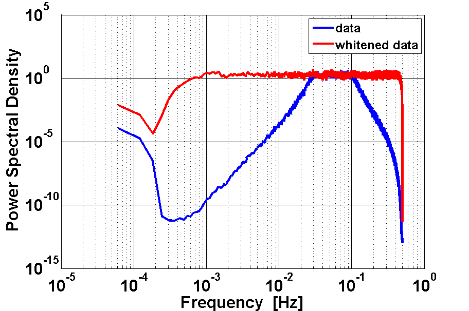
If you want to try buildWhitener1D to get a whitening filter for the present colored noise, you can try the following code. Please refer to the buildWhitener1D documentation page for the meaning of any parameter. The result of the whitening procedure is reported in figure 2.

      
    pl = plist(...
      'MaxIter', 30, ...
      'MinOrder', 9, ...
      'MaxOrder', 15, ...
      'FITTOL', 5e-2);
  
    wfil = buildWhitener1D(af,pl);

    aw = filter(af,wfil);

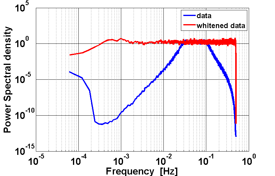
**Figure 2:** Power spectral density (estimated with the welch method) of colored and whitened processes.

Firwhiten

As an alternative you can try firwhiten to whiten the present colored noise. Please refer to the firwhiten documentation page for the meaning of any parameter. The result of the whitening procedure is reported in figure 3.

      
    pl = plist(...
      'Ntaps', 5000, ...
      'Nfft', 1e5, ...
      'BW', 5);
  
    aw = firwhiten(af, pl);

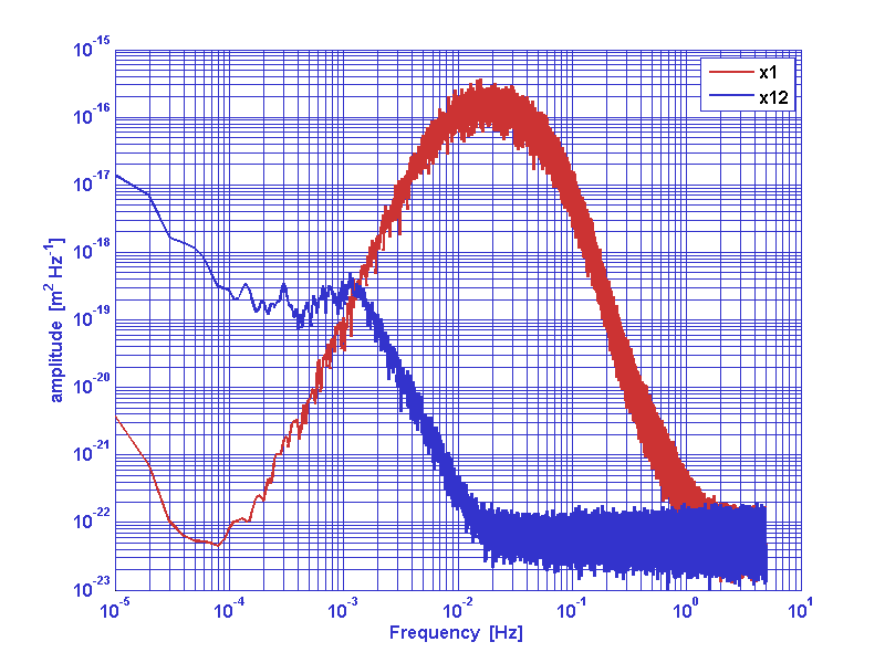
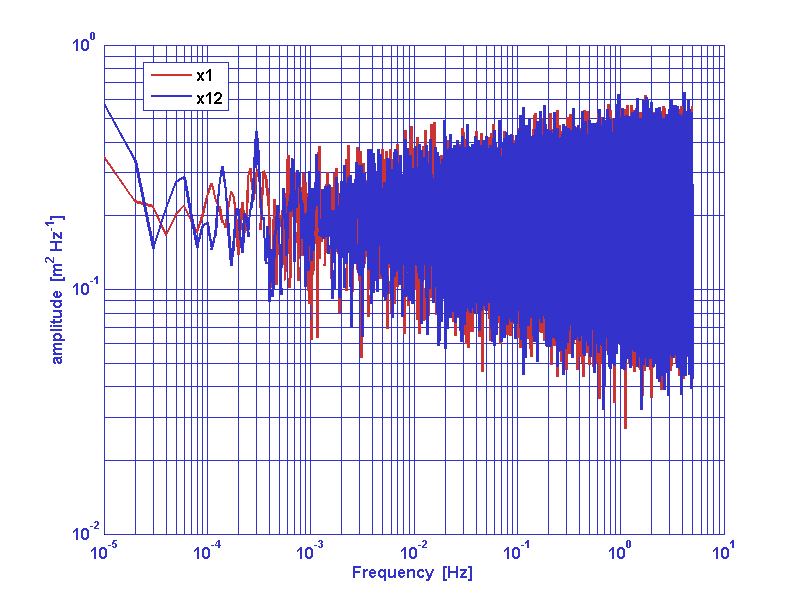
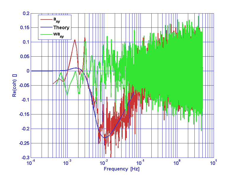
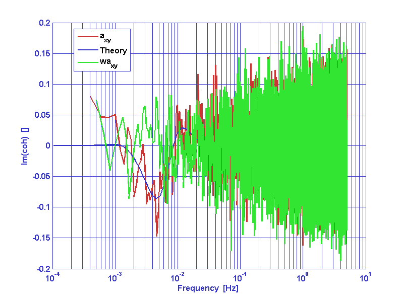
**Figure 3:** Power spectral density (estimated with the welch method) of colored and whitened processes.

Whitening noise in two-dimensional data

We consider now the problem of whitening cross correlated data series. As a example we consider a typical couple of x-dynamics LTP data series. a1 and a2 are interferometer output noise data series. In oreder to whiten data we must input a frequency response model of the cross spectral matrix of the cross-correlated process.

Refer to whiten2D documentation page for the meaning of any parameter.

      
    pl = plist(...
      'csd11', mod11, ...
      'csd12', mod12, ...
      'csd21', mod21, ...
      'csd22', mod22, ...
      'MaxIter', 75, ...
      'PoleType', 3, ...
      'MinOrder', 20, ...
      'MaxOrder', 40, ...
      'Weights', 2, ...
      'Plot', false,...
      'Disp', false,...
      'MSEVARTOL', 1e-2,...
      'FITTOL', 1e-3);
  
    [aw1,aw2] = whiten2D(a1,a2,pl);

**Figure 4:** Power spectral density of the noisy data series before (left) and after (right) the whitening.

**Figure 5:** Real (left) and Imaginary (right) part of the coherence function. Blue line refers to theoretical expectation for colored noise data. Red line refers to calculated values for colored noise data. Green line refers to calculated values for whitened noise data.

Data gap filling

Signal Processing in LTPDA