LTPDA Toolbox™

contents

Data gap filling

Description

Gaps in data can be filled with interpolated data if desired. LTPDA gapfilling joins two AOs by means of a segment of synthetic data. This segment is calculated from the two input AOs. Two different methods are possible to fill the gap in the data: linear and spline. The former fills the data by means of a linear interpolation whereas the latter uses a smoother curve ---see examples below.

Syntax

    

    b = gapfilling(a1, a2, pl)
  

where a1 and a2 are the two segments to join.

Parameters

• 'method' - method used to interpolate missing data (see below for details)
  • 'linear' (default option)
  • 'spline'
• 'addnoise' - with this option noise can be added to the interpolated data. This noise is defined as a
  random variable with zero mean and variance equal to the high-frequency noise of the input AO.

Algorithm

Linear : The gap is filled using a linear approximation.

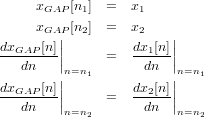
Spline : a third order interpolation is used in this case

The parameters a, b, c and d are calculated by solving next system of equations:

Examples

1. Missing data between two vectors of random data interpolated with the linear method.

      

  x1 = ao(plist('waveform','noise','nsecs',1e3,'fs',10,'name','noise')); % create an AO of random data
  xs = split(x1,plist('chunks',3));                              % split in three segments
  pl = plist( 'method',  'linear', 'addnoise', 'no');            % linear gapfilling
  y = gapfilling(xs(1),xs(3), pl);                               % fill between 2nd and 3rd segment
  iplot(x1,y) 
    

2. Missing data between two data vectors interpolated with the spline method.

      

  x1 = ao(plist('tsfcn','t.^1.8 + 1e6*rand(size(t))','nsecs',5e3,'fs',10,'name','noise')); % create an AO
  xs = split(x1,plist('chunks',3));                               % split in three segments
  pl = plist( 'method',  'spline', 'addnoise', 'no');             % cubic gapfilling
  y = gapfilling(xs(1),xs(3), pl);                                % fill between 2nd and 3rd segment
  iplot(x1,y) 
    

Spikes reduction in data

Noise whitening

©LTP Team