LTPDA Toolbox™

Transforming models between representations

Modelling a system

To show some of the possibilities of the toolbox to model digital system we introduce the usual notation for a closed loop model:

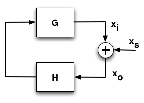
In our example we will assume that we know the pzmodel of the filter, H, and the open loop gain (OLG). These are related with the closed loop gain (CLG) by the following equation:

We want to determine G and CLG. We would also like to find a digital filter for H, but we will deal with this in the following section.

Loading the starting models

Imagine that we have somehow managed to find the following model for OLG:

Key	Value
`GAIN`	4e6
`POLES`	1e-6

then we can create a pzmodel with these parameters as follows

    OLG = pzmodel(4e6, 1e-6, [], 'OLG')
    ---- pzmodel 1 ----
           name: OLG
           gain: 4000000
          delay: 0
         iunits: []
         ounits: []
    description:
           UUID: 3d8bce32-a9a9-4e72-ab4d-183da69a9b5d
    pole 001: (f=1e-06 Hz, Q=NaN, ri=-6.283e-06)
    -------------------

To introduce the second model, the one describing H, we will show another feature of the pzmodel constructor. We will read it from a LISO file, since this contructor accepts this files as inputs. We can then type

    H = pzmodel('topic4/LISOfile.fil')
    ---- pzmodel 1 ----
           name: none
           gain: 1000000000
          delay: 0
         iunits: []
         ounits: []
    description:
           UUID: e683b32f-4653-474e-b457-939d33aeb63c
	pole 001: (f=1e-06 Hz, Q=NaN, ri=-6.283e-06)
    pole 002: (f=1e-06 Hz, Q=NaN, ri=-6.283e-06)
    zero 001: (f=0.001 Hz, Q=NaN, ri=-0.006283)
-------------------

and we see how the constructor recognizes and translates the poles and zeros in the file. The model gets the name from the file but we can easily change it to have the name of our model:

    H.setName();

According to our previous definition we can get the plant by dividing the OLG by H. We can do so directly when dealing with pzmodel objects since multiplication and division are allowed for these objects, then

    G = OLG/H
    ---- pzmodel 1 ----
           name: (OLG./H)
           gain: 0.004
          delay: 0
         iunits: []
         ounits: []
    description:
           UUID: fcd166f7-d726-4d39-ad2e-0f3b7141415b
	pole 001: (f=1e-06 Hz, Q=NaN, ri=-6.283e-06)
	pole 002: (f=0.001 Hz, Q=NaN, ri=-0.006283)
	zero 001: (f=1e-06 Hz, Q=NaN, ri=-6.283e-06)
	zero 002: (f=1e-06 Hz, Q=NaN, ri=-6.283e-06)
    -------------------

which we need to simplify to get rid of cancelling poles and zeros. We also set the model name here.

    G.setName();
    G.simplify
    ---- pzmodel 1 ----
           name: simplify(G)
           gain: 0.004
          delay: 0
         iunits: []
         ounits: []
    description:
           UUID: c1883713-b860-4942-a127-e42ea565460f
	pole 001: (f=0.001 Hz, Q=NaN, ri=-0.006283)
	zero 001: (f=1e-06 Hz, Q=NaN, ri=-6.283e-06)
    -------------------

The CLG requires more than a simple multiplication or division between models and we will not be able to derive a pzmodel for it. However, we can evaluate the response of this object as follows:

    pl = plist('f1', 1e-3, 'f2', 5, 'nf', 100);
    CLG = 1/(1-resp(OLG, pl));
    CLG.setName();
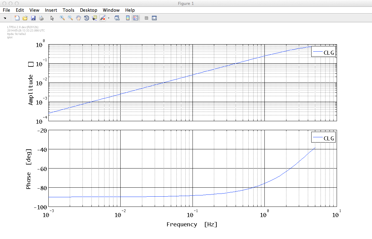
    CLG.iplot();

which gives us an AO that we can plot:

Fine, but my (real) system has a delay...

You can now repeat the same procedure but loading a H model with a delay from the LISO file 'LISOFileDelay.fil':

    H_Delay = pzmodel('topic4/LISOfileDelay.fil')
    ---- pzmodel 1 ----
           name: none
           gain: 1000000000
          delay: 0.125
         iunits: []
         ounits: []
    description:
           UUID: 6dfbddc5-b186-4405-8f6e-02a2822a22c5
	pole 001: (f=1e-06 Hz, Q=NaN, ri=-6.283e-06)
	pole 002: (f=1e-06 Hz, Q=NaN, ri=-6.283e-06)
	zero 001: (f=0.001 Hz, Q=NaN, ri=-0.006283)
    -------------------

and calculate the response:

    H_Delay.setName();
    pl = plist('f1', 1e-3, 'f2', 5, 'nf', 100);
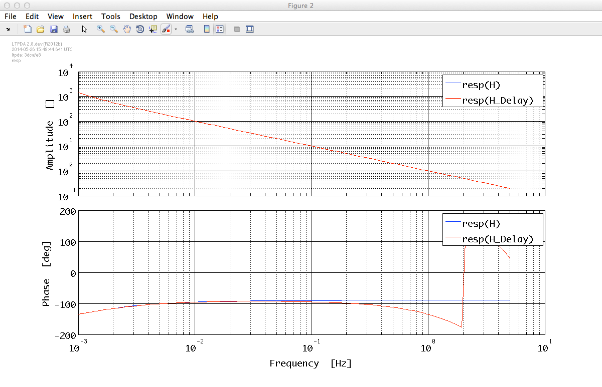
    resp([H, H_Delay], pl)

You will see how the delay is correctly handled, meaning that it is added when we multiply two models and subtracted if the models are divided.

Transforming models between representations

How to filter data