LTPDA Toolbox™

Whitening noise

The LTPDA toolbox offers various ways in which you could whiten data. Perhaps you know the whitening filter you want to use, in which case you can build the filter and filter the data using the method ao/filter. Alternatively, you may have a model for the spectral content of the data, in which case you can use the method ao/whiten1D if you are dealing with single, uncorrelated data streams, or ao/whiten2D if you have a pair of correlated data streams. You can also use ao/whiten1D in the case where you don't have a model for the spectral content of the data. In this case, the method calculates the spectrum of the data, re-bins the spectrum so to reduce the individual points fluctuations, and fits a model of the spectrum as a series of partial fractions z-domain filters.

The whitening algorithms are highly configurable and accept a large number of parameters. The main ones that we will change from the defaults in the following examples are

Key	Description
`PLOT`	Plot the result of the fitting as it proceeds.
`MAXORDER`	Specify the maximum allowed model order that can be fit.
`WEIGHTS`	Choose the way the data is weighted in the fitting procedure.
`RMSVAR`	Check if the variation of the RMS error is smaller than 10^(-b), where b is the value given in the plist.

We will start by whitening some data using this last method, i.e., allowing whiten1D to determine the whitening filter from the data itself.

The data we will whiten can be found in your data packet in the 'topic2' sub-directory.

We start by loading the mat file:

    a = ao('topic2/whiten.mat');

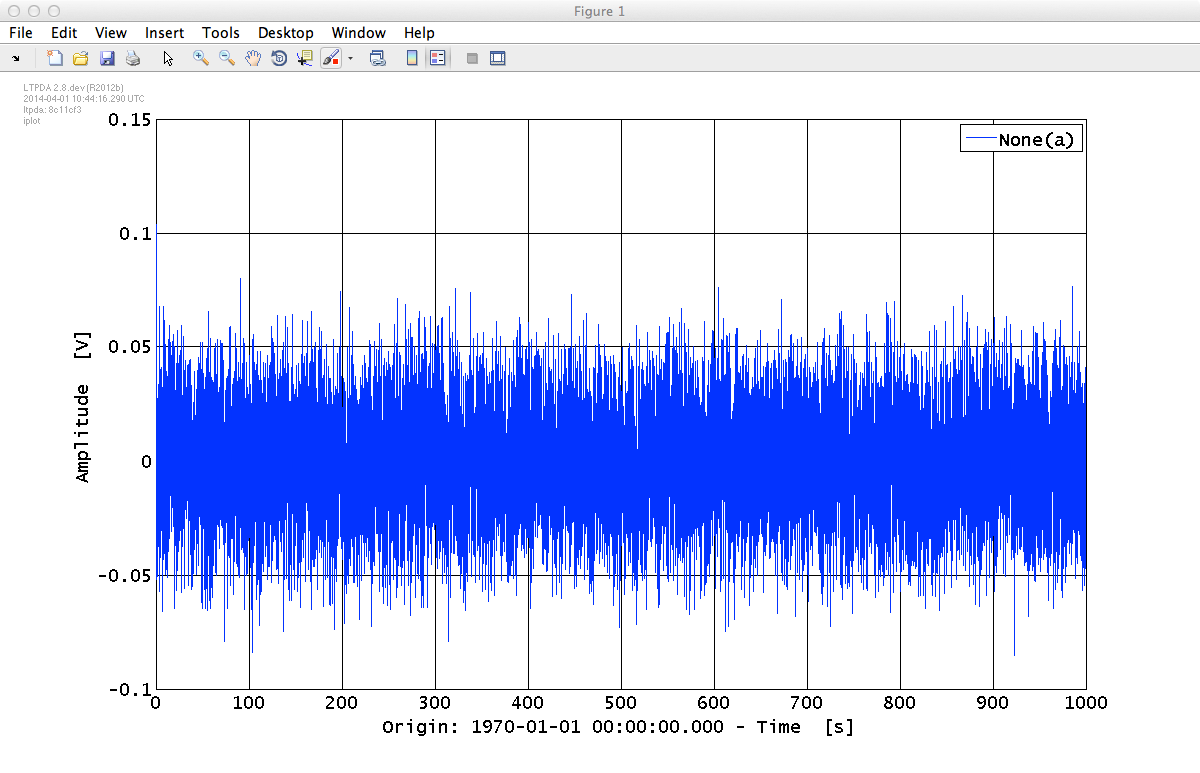
The AO stored in the variable a is a coloured noise time-series. Let's have a look at this times series using iplot.

    >> iplot(a);

The result should be similar to:

Before we can whiten the data, we have to define the parameter list for the whitening tool:

    pl = plist(...
              'Plot', true, ...
              'MaxOrder', 9, ...
              'Weights', 2);

Now we can call the whitening function whiten1D with our input AO, a and the parameter list pl:

 >> aw = whiten1D(a, pl);

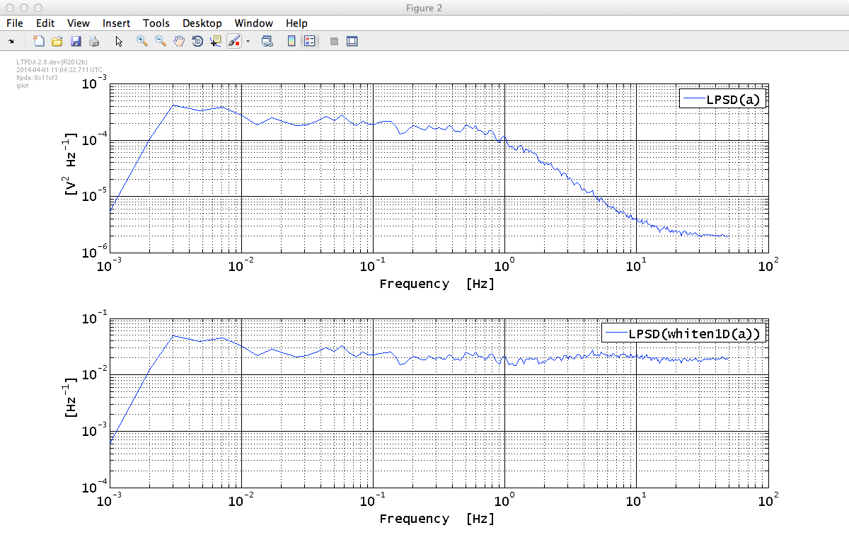
To compare the whitened data with the coloured noise we compute the power spectrum (for details see Power spectral density estimation):

    awxx = aw.lpsd;
    axx  = a.lpsd;

and finally plot our result in the frequency domain; in particular we plot the whitened data (awxx) compared to the coloured noise that was our input (axx). Please notice the choice of showing the whitened and colored data in two independent subplots, so to exploit their different range of values. Additionally, the units of the whitened data are reset to empty by the method, since the 'application' of the units is delegated to the whitening filter which is calculated as an intermediate step of the process.

    iplot(axx, awxx, plist('arrangement', 'subplots'));

Remove trends from a time-series AO

Select and find data from an AO