

| LTPDA Toolbox™ | contents | |
The ao class has a method for interpolating data using different forms of interpolation. This method is called ao/interp.
To configure ao/interp, use the following parameters:
| Key | Description |
|---|---|
|
VERTICES |
A new set of vertices (relative to the data reference time t0) on which to resample. |
|
METHOD |
The method by which to interpolate. Choose from
|
Here we will interpolate a sinusoidal signal on to a new time-grid. The result will be to increase the sample rate by a factor 2.
First we create a time-series ao:
    pl = plist('Name', 'None', 'tsfcn', 'sin(2*pi*1.733*t)', 'fs', 20, 'nsecs', 10, 'yunits', 'V');
    x  = ao(pl);
Then we create the new time-grid we want to resample on to.
tt = linspace(0, x.nsecs - 1/x.fs, 2*(x.len));
Please notice the 'dot' notation we used to call a couple methods to access properties of this tsdata (time-series) AO:
x.nsecs
x.fs
Finally, we can apply our new time-grid to the data using interp. We test two of the available interpolation methods:
    pl_spline  = plist('vertices', tt);
    pl_nearest = plist('vertices', tt, 'method', 'nearest');
    x_spline   = interp(x, pl_spline);
    x_nearest  = interp(x, pl_nearest);
    iplot(x, x_spline, x_nearest, plist('Markers', {'o', '+', 'x'}, ...
    'LineColors', {'k', 'r', 'g'}, ...
    'XRanges', [0 1]));
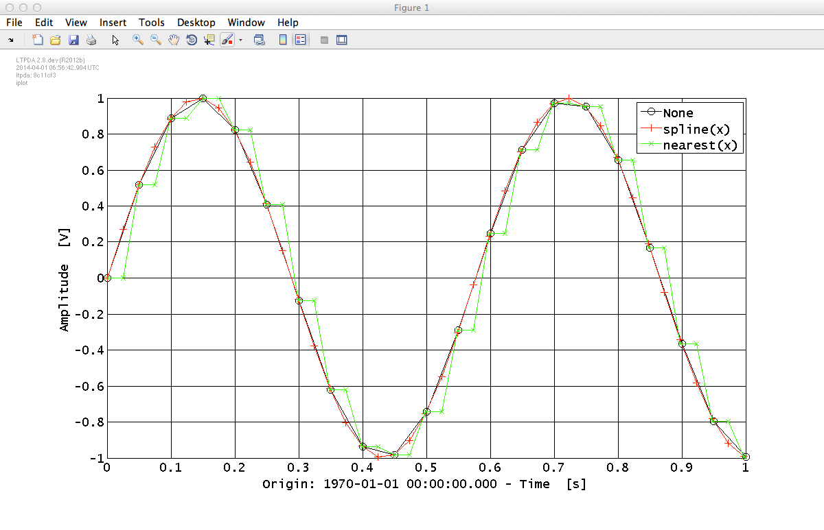
Notice the settings in the plist we used for the plotting, that allow changing the marker of the plotted lines, as well as the settings for adjusting the colors of the line themselves.
| |
Resampling a time-series AO | Remove trends from a time-series AO | |
©LTP Team