

| LTPDA Toolbox™ | contents | |
params = {...
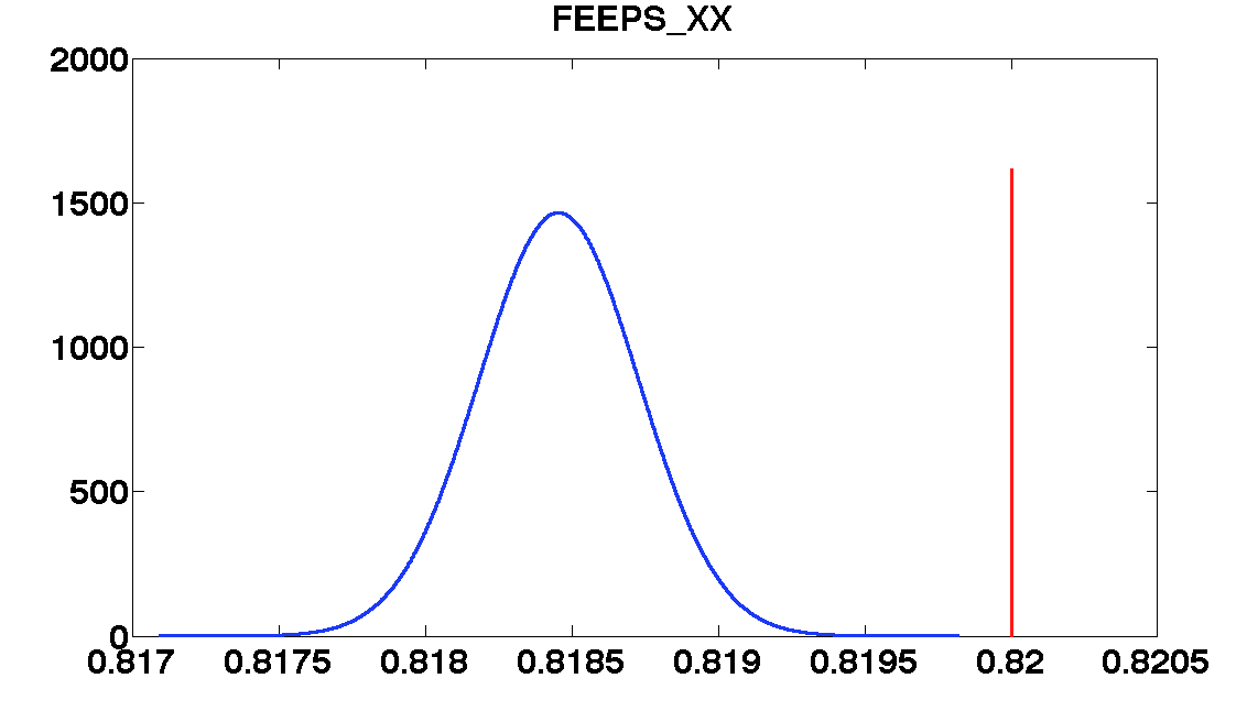
'FEEPS_XX', ...
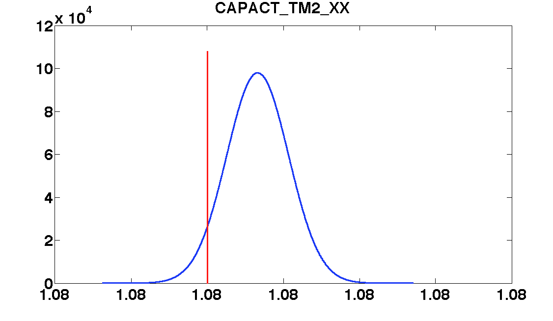
'CAPACT_TM2_XX', ...
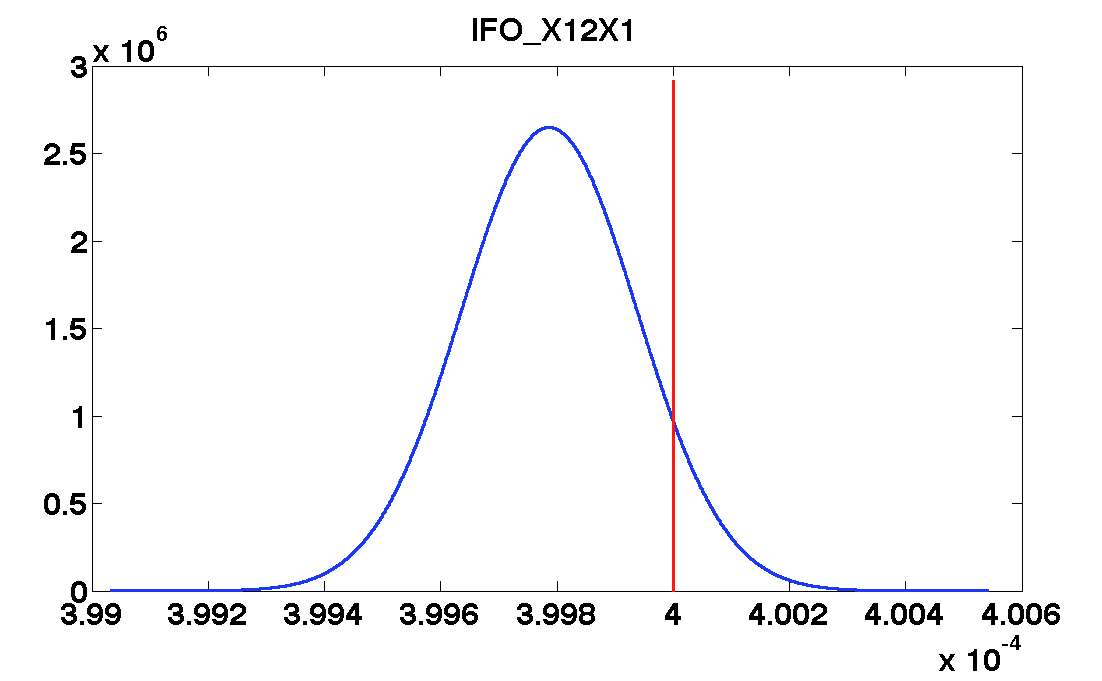
'IFO_X12X1', ...
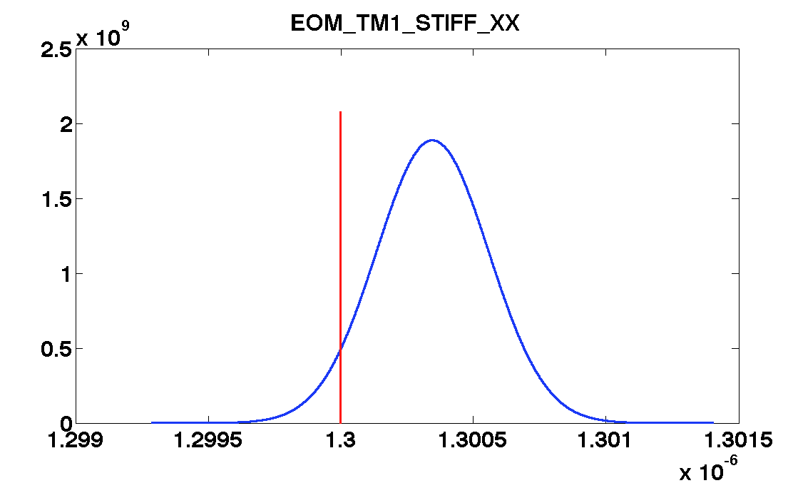
'EOM_TM1_STIFF_XX', ...
'EOM_TM2_STIFF_XX'};
values = [0.82 1.08 0.0004 1.3e-6 1.9e-6];
plshow = plist(...
'FitParams', params,...
'FitParamsValues', values);
linfitsvdPlot(fpars, plshow);
pl = plist(...
'burnin', 1000, ... % The number of samples to be discarded from the chain
'pdfs', true, ... % Plot the pdfs of the parameters
'chain', 0 ,... % Do not plot chains
'separate pdfs', [1 2 3 4 5], ... % Plot the pdfs in separate figures
'nbins', 20, ... % Number of bins for the histograms
'colormap', summer, ... % choose colormap for cosmetics!
'results', true); % Print results to screen
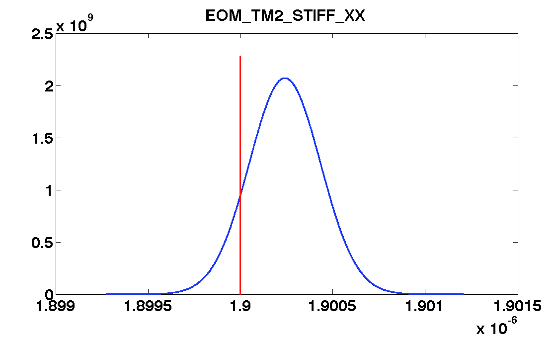
mcmcPlot(b,pl)
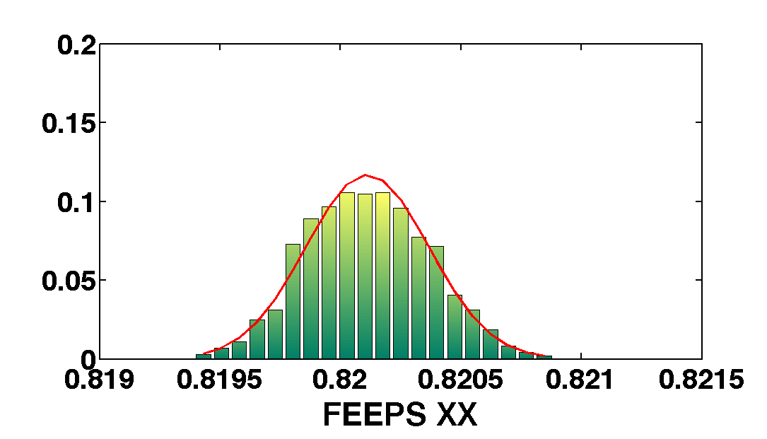
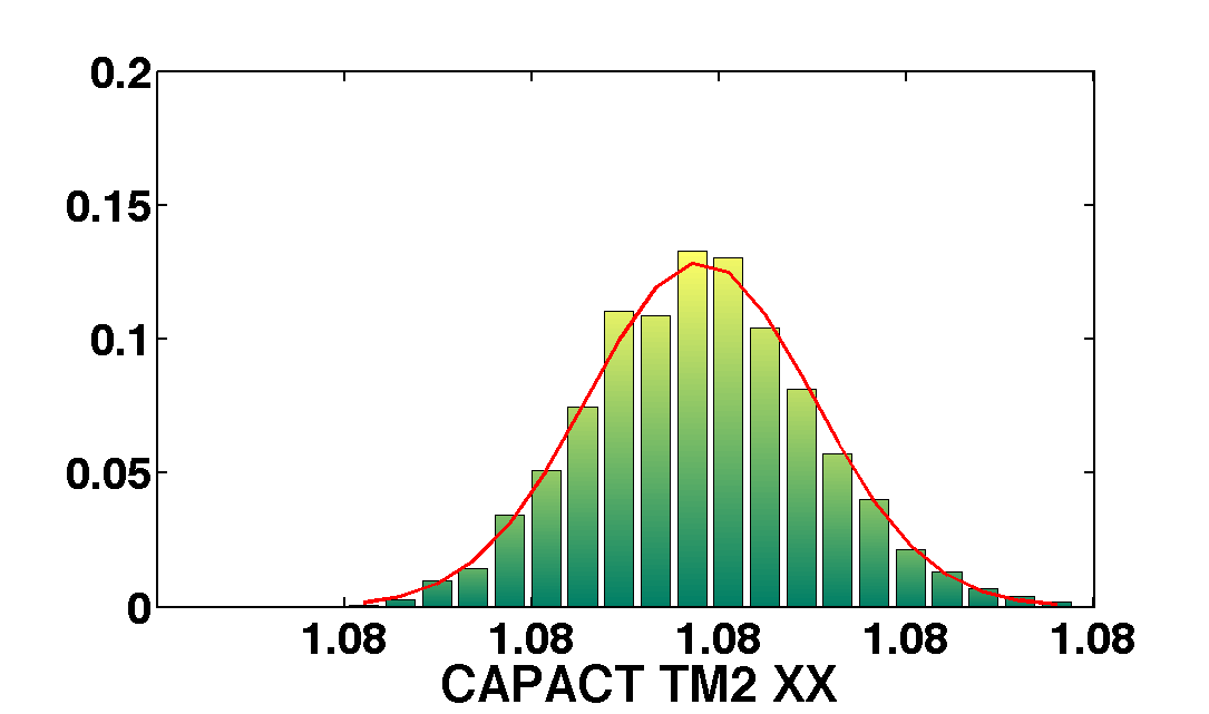
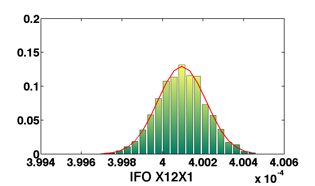
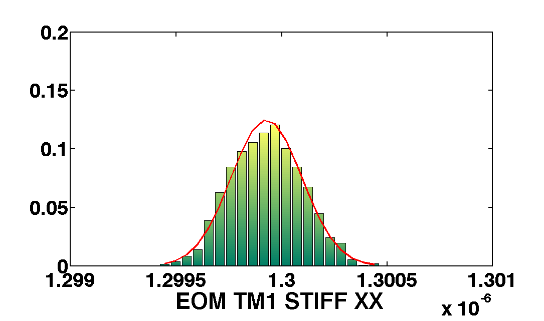
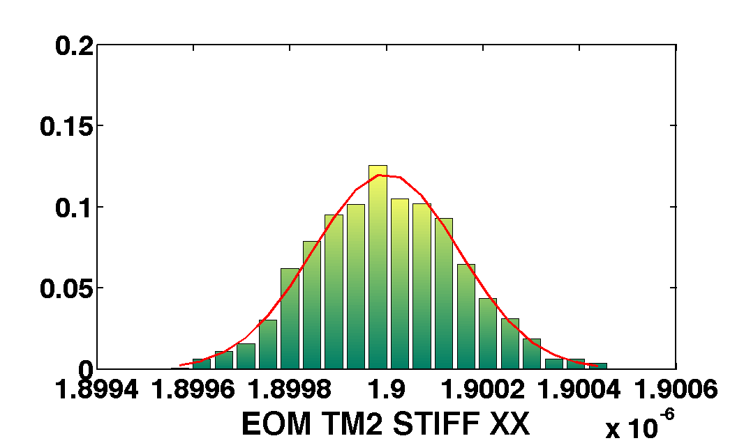
The table below show the comparison of the results obtained with the two methods. We compare as well the error on the parameter with the optimal error expected from the Fisher matrix analysis
| Parameter | True value | Exp. error | Linear | MCMC |
|---|---|---|---|---|
| FEEPS_XX | 0.82 | 0.0002 | 0.8185 ± 3e-4 | 0.8201 ± 2.5e-04 |
| CAPACT_TM2_XX | 1.08 | 3.0e-06 | 1.080007 ± 4e-06 | 1.080004 ± 3e-06 |
| IFO_X12X1 | 0.0004 | 1.1e-07 | 3.998e-04 ± 1.5e-07 | 4.000e-04 ± 1e-07 |
| EOM_TM1_STIFF_XX | 1.3e-6 | 1.7e-10 | 1.3004e-06 ± 2.0e-10 | 1.2999e-06 ± 1.6e-10 |
| EOM_TM2_STIFF_XX | 1.9e-6 | 1.6e-10 | 1.9002e-06 ± 2.0e-10 | 1.8999e-06 ± 1.5e-10 |
| |
Linear Parameter Estimation | Use parameter estimates to estimate residual differential acceleration | |
©LTP Team