Building whitening filters (LTPDA Toolbox)

Whitening filters can be constructed from power spectral density (PSD) of noise only data series. The procedure can be summarized in few steps:

    noise = matrix('noise.mat');

Assuming the noise is stationary we calculate whitening filter from the noise only part of the first experiment.

    [n1, n2] = noise(1).unpack;

Whitening filter will be calculated from the noise spectra. We assume that the correlations between the two data series are so low that they cannot be properly identified by a cpsd estimation. Therefore we calculate two independent whitening filters for the two output channels. This is equivalent to assume uncorrelated data.

    n1x = n1.lpsd;
    n2x = n2.lpsd;

    n1xx = split(n1x, plist('samples', [6 numel(n1x.y)]));
    n2xx = split(n2x, plist('samples', [6 numel(n2x.y)]));

    iplot(n1xx, n2xx)

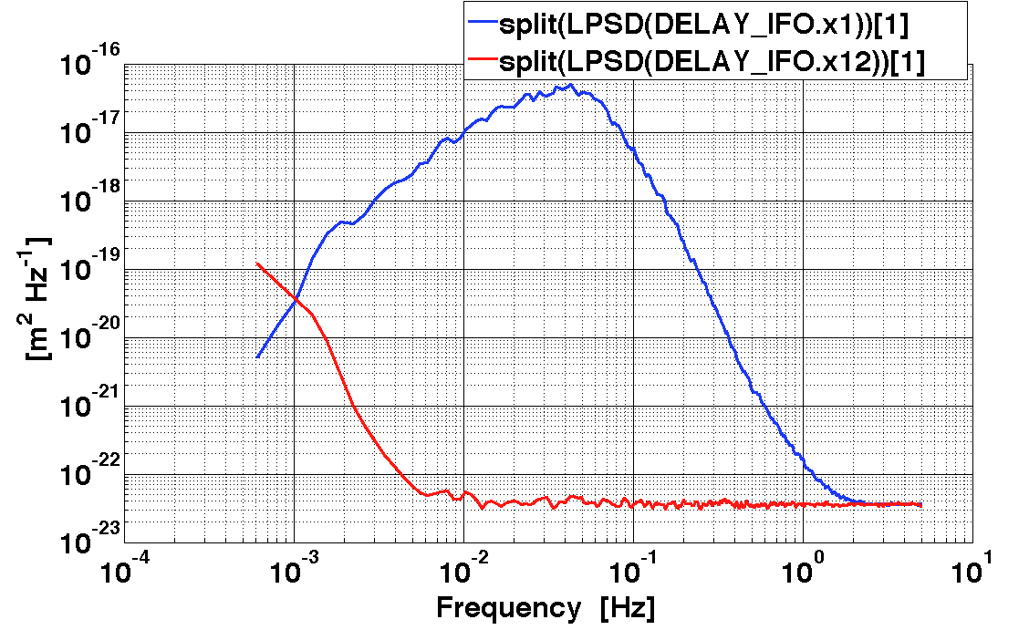
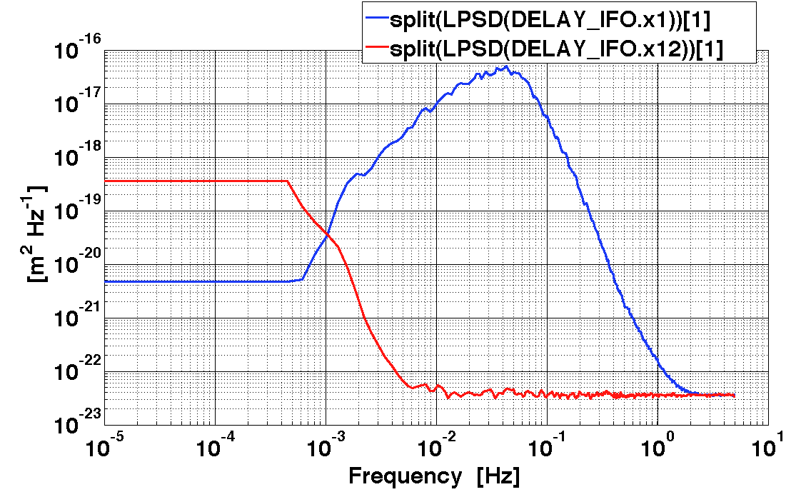
Since the amount of data is limited, we do not properly cover low frequency with the estimated spectrum. We need to exted low frequency part in order to avoid that the fit would introduce unwanted features in a sensible frequency range (e.g. if we skip this part we end-up with a notch on channel 1 that will be clearly visible in the whitened time series).

    xt = [logspace(-5, log10(4.5e-4), 60)]';
    
    level1 = n1xx.y(1) .* 0.90;
    yt1 = ones(numel(xt),1) .* level1;

    level2 = n2xx.y(1) .* 3.00;
    yt2 = ones(numel(xt),1) .* level2;

    yunit  = n1xx.yunits;
    fs     = n1xx.fs;    
    ext1   = ao(plist('XVALS', xt, 'YVALS', yt1, 'TYPE', 'FSDATA', 'YUNITS', yunit, 'FS', fs));
    ext2   = ao(plist('XVALS', xt, 'YVALS', yt2, 'TYPE', 'FSDATA', 'YUNITS', yunit, 'FS', fs));

    nn1xx = join(ext1, n1xx);
    nn2xx = join(ext2, n2xx);

    iplot(nn1xx, nn2xx)

In order to obtain a smooth version of the calculated PSD we perform a frequency domain fit with the 'ao' class method 'sDomainFit', which output a 'parfrac' object that can be used to define the input for our whitener.

      
      plfit = plist(...
                'AUTOSEARCH', 'on', ...
                'STARTPOLESOPT', 'clog', ...
                'maxiter', 30, ...
                'minorder', 4, ...
                'fittol', 1e-2, ...
                'msevartol', 5e-1, ...
                'plot', 'off');
      
      s1 = sDomainFit(nn1xx,plfit);
      
      
      
      plfit = plist(...
                'AUTOSEARCH', 'on', ...
                'STARTPOLESOPT', 'clog', ...
                'maxiter', 30, ...
                'minorder', 3, ...
                'fittol', 1e-2, ...
                'msevartol', 5e-1, ...
                'plot', 'off');
      
      s2 = sDomainFit(nn2xx,plfit);

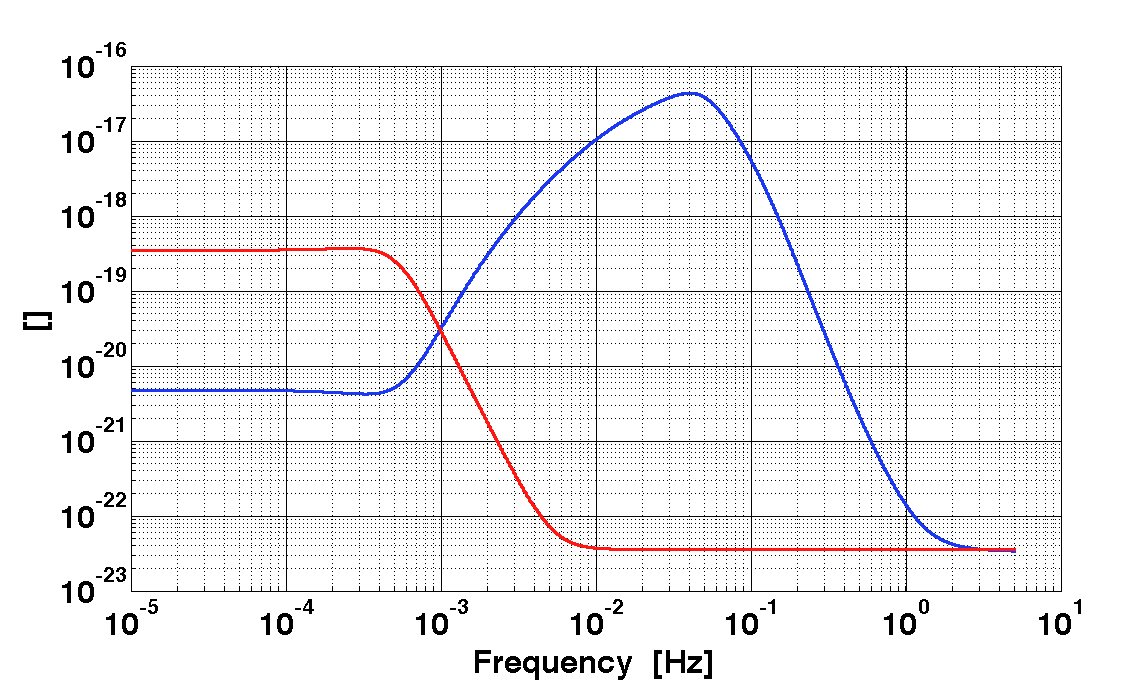
Frequency series 'aos' can be constructed from the 'parfrac' objects. They will be used as input to 'buildWhitener'.

    plr  = plist('f',logspace(-5, log10(5), 5000)); % define plist with frequency grid

    rs1  = s1.resp(plr); % get frequency response from parfarc object
    mod1 = abs(rs1); % this is a model for a psd, so it must be real

    rs2  = s2.resp(plr); % get frequency response from parfarc object
    mod2 = abs(rs2); % this is a model for a psd, so it must be real

    iplot(mod1,mod2)

We are now ready to build the whitening filters for the first and differential channels. 'buildWhitener', build a whitening filter from a frequency series input and a 'plist'. The frequency series 'ao' should be representative of the one-sided psd of the noise we want to whiten. 'buildWhitener' perform a fit in the z-domain to the data in order to identify the coefficients (poles and residues) of a digital filter.

    
    plw = plist(...
          'fs', fs,...
          'FITTOL', 1e-3);

    w1 = buildWhitener1D(mod1, plw);
    w2 = buildWhitener1D(mod2, plw);

  
    help ao/buildWhitener1D

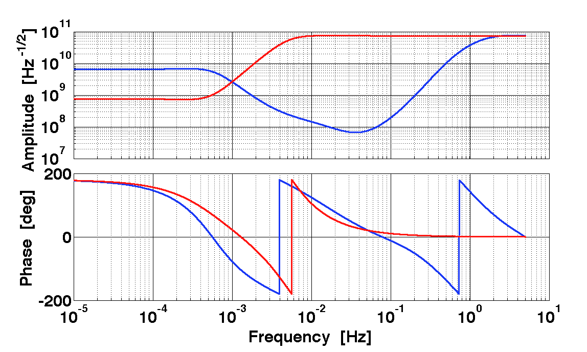
Once we have the whitening filters, we can check their frequency response. It is good practice to ceck filters response on a frequency grid tighter than that used for buildind the filter.

  
    plr = plist('f', logspace(-5, log10(5), 10000));

    rw1 = w1.resp(plr);
    rw2 = w2.resp(plr);

    iplot(rw1,rw2)

  
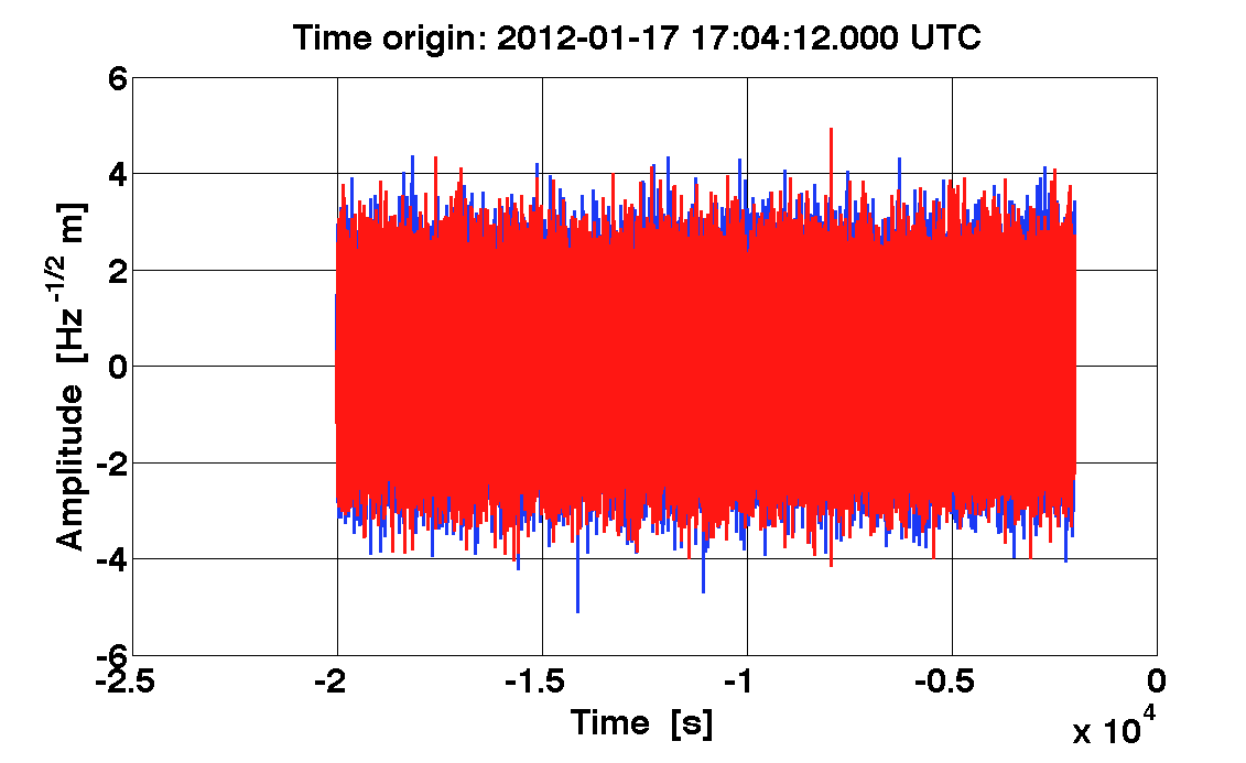
    nw1 = filter(n1, w1);
    nw2 = filter(n2, w2);

    iplot(nw1, nw2)

  
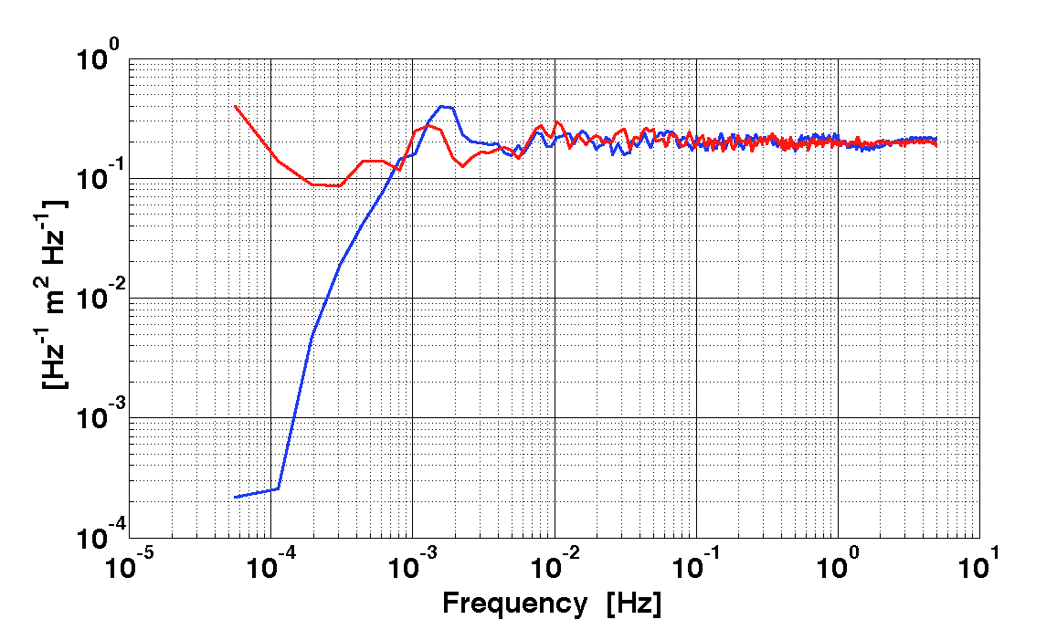
    nw1xx = lpsd(nw1);
    nw2xx = lpsd(nw2);

    iplot(nw1xx, nw2xx)

Once we are happy with our whitening filters, we can pack them in a matrix (diagonal) and save it. In order to have a diagonal filter matrix we will put empty filter objects out of the diagonal.

  
    % out of diagonal filter
    fil = filterbank(miir());

    % build a matrix with whitening filters elements
    wf = matrix(w1, fil, fil, w2, plist('shape', [2 2]));
    
    wf.save('whitening_filter.mat');