

| LTPDA Toolbox™ | contents | |
We can, of course, do the same injections but with the full LPF model and with noise switched on.
In Topic 2 you already saw how to simulate an LPF model with all the noises switched on. If we combine that with the signal injections we've been doing in this topic, then a simulation with noise and injected signals can be done like this:
      % Create a standard LPF model
      lpf = ssm(plist('built-in', 'LPF'));

      % Generate suitable covariance matrix for all inputs
      cov = lpf.generateCovariance;

      % Create some time-series analysis object to inject
      aSignal = ao(plist('tsfcn', '1e-7*sin(2*pi*0.005*t)', 'fs', 1/lpf.timestep, 'nsecs', 10000));

      % Create the plist to configure simulate
      sim_pl = plist('AOS', aSignal, 'AOS Variable Names', 'GUIDANCE.ifo_x1', ...
                     'return outputs', {'DELAY_IFO.x1', 'DELAY_IFO.x12'}, ...
                     'CPSD variable names', cov.find('names'), ...
                     'CPSD', cov.find('cov'));

      % Run the simulation
      out = simulate(lpf, sim_pl);
% Unpack the outputs
[o1, o12] = unpack(out);
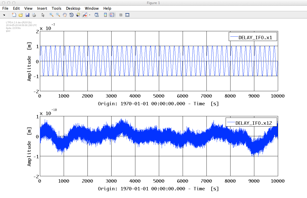
% Plot on subplots
plot_pl = plist('arrangement', 'subplots');
iplot(o1, o12, plot_pl);
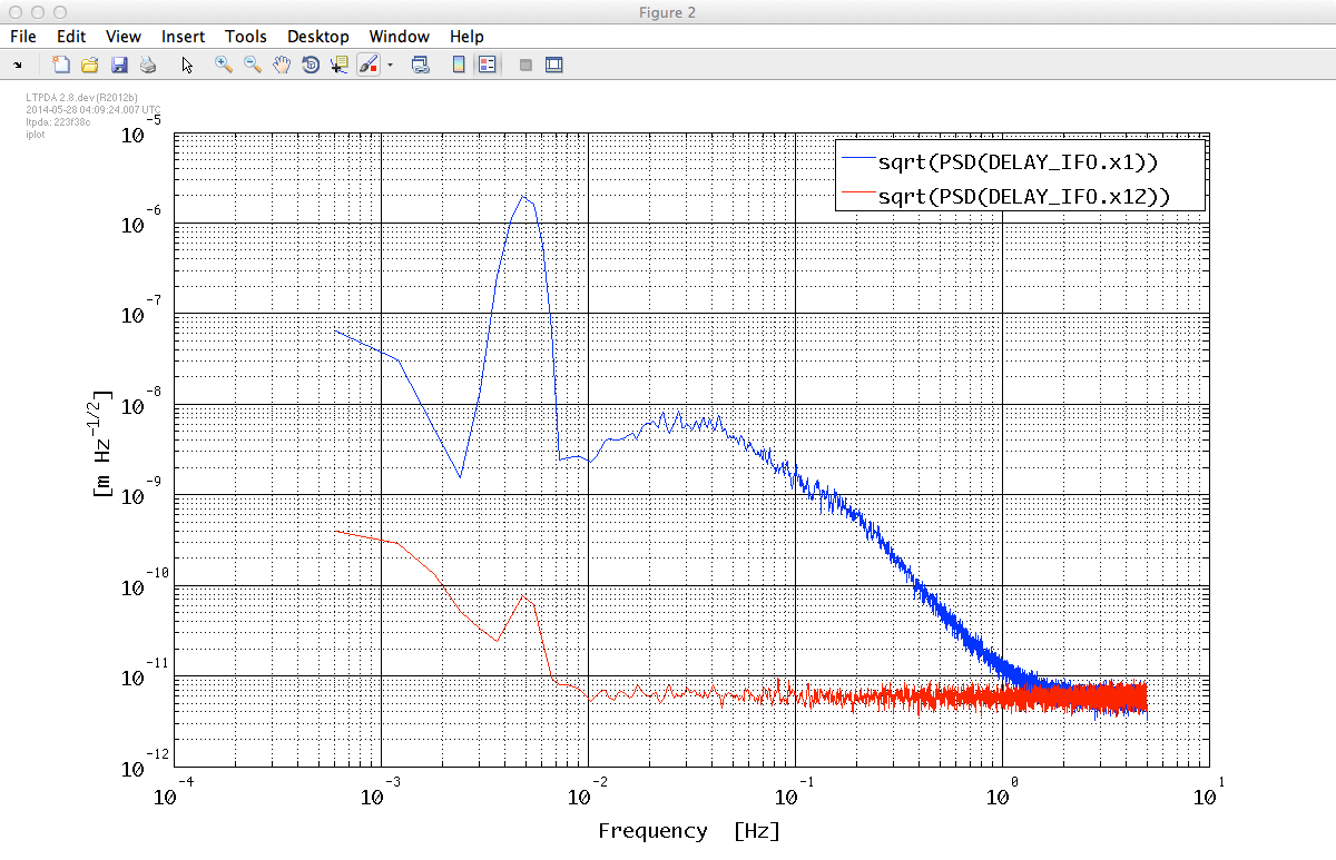
      % Create a PSD plist with 16 averages, linear segment-wise detrending
      psd_pl = plist('navs', 16, 'order', 1, 'win', 'BH92');

      % Estimate PSDs
      [o1_xx, o12_xx] = psd(o1, o12, psd_pl);

      % Plot the ASDs
      iplot(sqrt(o1_xx), sqrt(o12_xx));
| |
Estimate tranfser functions from simulated signals, compare with Bode estimates | Topic 5 - Introduction to system identification of LPF. | |
©LTP Team