

| LTPDA Toolbox™ | contents | |
We can estimate transfer functions of the system in two ways: by injecting noise and using spectral estimator methods, or by computing the Bode response based on the system matrices.
Let's start by injecting a white noise time-series in to the guidance input of the y1 control coordinate:
      % Create a noise time-series analysis object to inject
      fs    = 1/ltp.timestep;
      nsecs = 10000;
      noise = ao.randn(nsecs, fs);
      noise.setYunits('m'); % We want to inject [m]. Then the estimated TF later will have the right units.
      noise.setName;

      % Generate a list of outputs we want from the simulator
      outputs = ltp.getPortNamesForBlocks(plist('blocks', {'DELAY_IFO', 'IS'}, 'type', 'outputs'));

      % Create the plist to configure simulate
      sim_pl = plist('AOS', noise, 'AOS Variable Names', 'GUIDANCE.is_tm1_y', 'return outputs', outputs)

      % Run the simulation
      out = simulate(ltp, sim_pl);
      % Create a plist to configure iplot to plot with subplots
      plot_pl = plist('arrangement', 'subplots');

      % First extract the internal AOs we want and then plot
      IS_tm1_y = out.getObjectAtIndex(8);
      IS_tm2_y = out.getObjectAtIndex(14);

      % Then plot the IS y signals together
      iplot(IS_tm1_y, IS_tm2_y, plot_pl);
      tfe_pl = plist('navs', 16, 'order', 1, 'win', 'BH92');
      Tn2is1y = tfe(noise, IS_tm1_y, tfe_pl);
iplot(Tn2is1y);
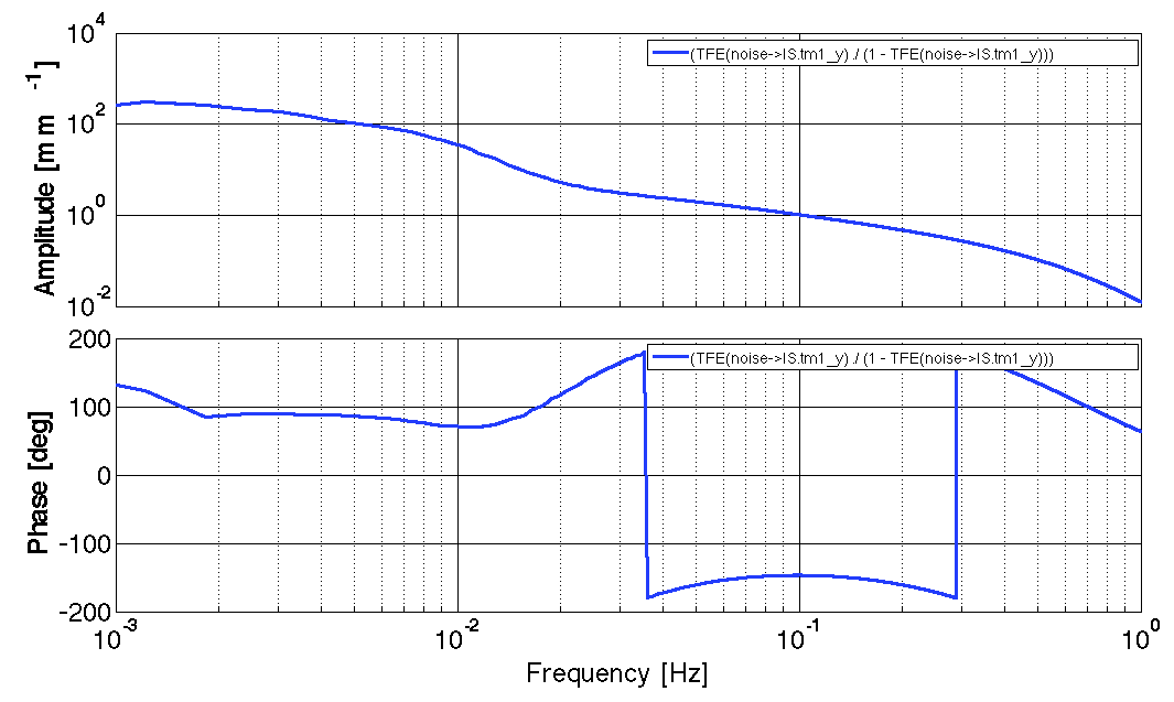
O = Tn2is1y / (1 - Tn2is1y)
iplot(O, plist('xranges', {'all', [1e-3 1]}));
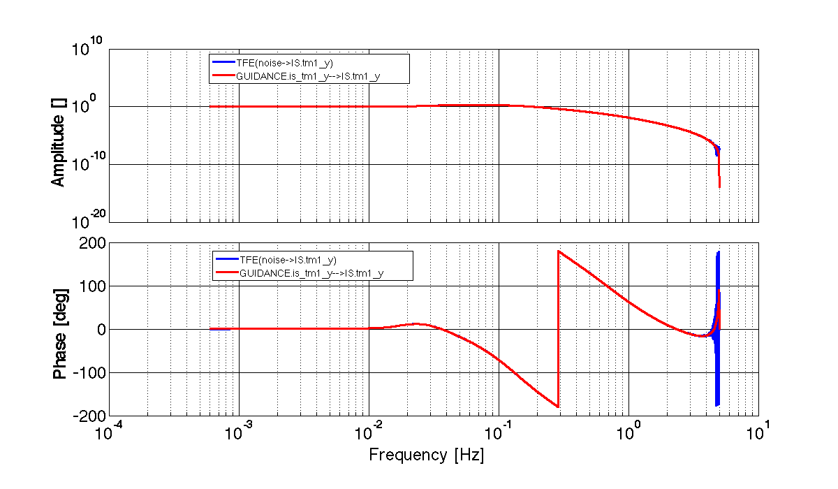
We can also extract transfer functions from the system directly using the ssm/bode function. The usage of the bode method is very similar to simulate. You have to specify the input and output ports, and a set of frequencies to compute the response at, and bode returns one frequency-series for each possible input to output transfer function.
Using the same LTP model we've been using all along, you can extract the same transfer function as the one measured above by doing:
      % Create a plist to configure bode. Evaluate the response at the frequencies of the measured TF from above.
      bpl = plist('inputs', 'GUIDANCE.is_tm1_y', 'outputs', 'IS.tm1_y', 'f', Tn2is1y.x);

      % Compute the response
      out = bode(ltp, bpl);
      Tb = out.getObjectAtIndex(1);
      iplot(Tn2is1y, Tb);
| |
Inject noise signals to LTP | Simulate LPF with injected signals | |
©LTP Team