Simulations (LTPDA Toolbox)

>> sys = ssm(plist('built-in', 'standard_system_params', 'setnames', {'W' 'C'}, 'setvalues', [-0.2 -0.5]));
>> sys.modifTimeStep(0.01);
>> sys.duplicateInput('U','Negative Bias');
>> controller = ssm(plist( ...
'amats',cell(0,0), 'bmats',cell(0,1), 'cmats',cell(1,0), 'dmats',{-1}, ...
'timestep',0.01, 'name','controller', 'params',plist, ...
'statenames',{}, 'inputnames',{'Y'}, 'outputnames',{'U'} ));
------ ssm/1 -------
      amats: {  [2x2]  }  [1x1]
      mmats: {  [2x2]  }  [1x1]
      bmats: {  [2x2]   [2x1]  }  [1x2]
      cmats: {  [1x2]   
                [1x2]  }  [2x1]
      dmats: {  [1x2]    []     
                [1x2]    []    }  [2x2]
   timestep: 0.01
     inputs:  [1x2 ssmblock]
         1 : N | Fn [kg m s^(-2)], On [m]
         2 : Negative Bias | Fu [kg m s^(-2)]
     states:  [1x1 ssmblock]
         1 : standard test system | x [m], xdot [m s^(-1)]
    outputs:  [1x2 ssmblock]
         1 : Y | y [m]
         2 : U | U > 1 []
     params: (empty-plist) [1x1 plist]
    version: $Id$
    Ninputs: 2
 inputsizes: [2 1]
   Noutputs: 2
outputsizes: [1 1]
    Nstates: 1
 statesizes: 2
    Nparams: 0
isnumerical: true
       hist: ssm.hist [1x1 history]
   procinfo: (empty-plist) [1x1 plist]
   plotinfo: (empty-plist) [1x1 plist]
       name: assembled( standard_system_params + controller))
description: 
    mdlfile: 
       UUID: 163d7103-063b-4a57-af7e-b08d22fe42c1
--------------------

Then we wish to use the inputs of N for a correlated force noise and measurement noise, “Negative Bias” for a sinewave, and there will be an observation DC offset.

We want as an output the controller output “U” and the sensor output “y”.

>> ao1 = ao(plist('FCN','sin(0:0.01:100)'));
>> ao_out = sysCL.simulate( plist(...
 'NOISE VARIABLE NAMES', {'Fn' 'On'}, 'COVARIANCE', [1 0.1 ; 0.1 2] , ...
 'AOS VARIABLE NAMES', {'Fu'} ,'AOS', ao1 ,...
 'CONSTANT VARIABLE NAMES', {'On'}, 'CONSTANTS', 35, ...
 'RETURN STATES', {'x'}, 'RETURN OUTPUTS', {'y' 'U > 1'}, ...
 'SSINI' , {[100;3]}, 'TINI', 0));
>> iplot(ao_out([1, 2, 3]));

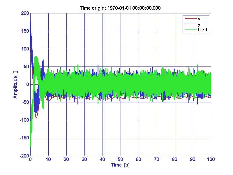
It turns out the system output (blue) is not much like the state (red), causing the control (green) to waste a lot of energy. The state is not experimentally available, but might be obtained through filtering. The kalman method is so far the only filtering method implemented in the toolbox.

>> ao_est = sysCL.kalman( plist(...
 'NOISE VARIABLE NAMES', {'Fn' 'On'}, 'COVARIANCE', [1 0.1 ; 0.1 2] , ...
 'AOS VARIABLE NAMES', {'Fu'} ,'AOS', ao1 ,...
 'CONSTANT VARIABLE NAMES', {'On'}, 'CONSTANTS', 35, ...
 'OUTPUT VARIABLE NAMES', {'y'}, 'OUTPUTS' , ao_out(2), ...
 'RETURN STATES', 1, 'RETURN OUTPUTS', 1 ));
>> iplot(ao_out(2), ao_est(1), ao_out(1))

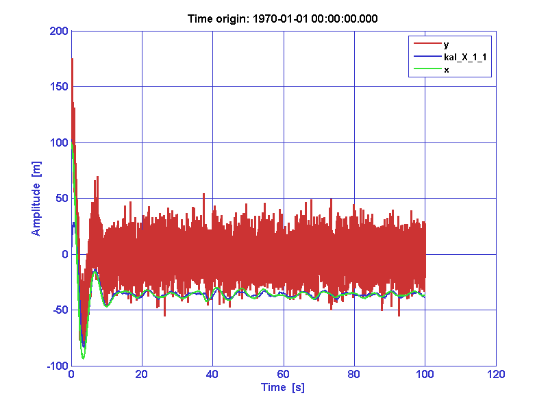
In this example the estimate (blue) of the state (green) is satisfactory. It leads us to think that such a filter should be used to provide with the input of the controller.

However, the DC offset correction by the kalman filter is one information that is not available under usual circumstances.

Simulations

Simulation example.