

| LTPDA Toolbox™ | contents | |
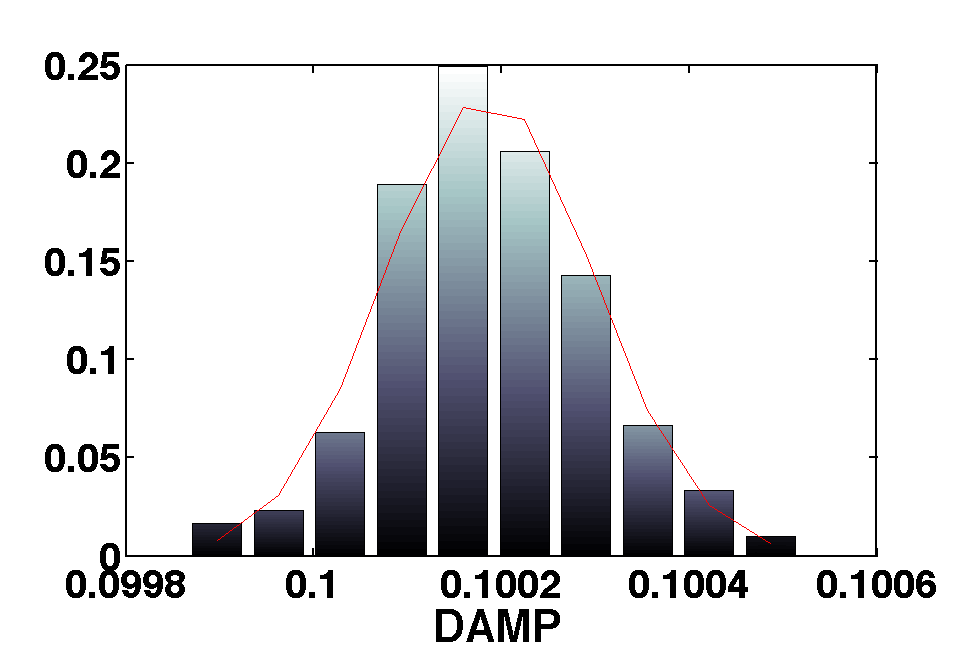
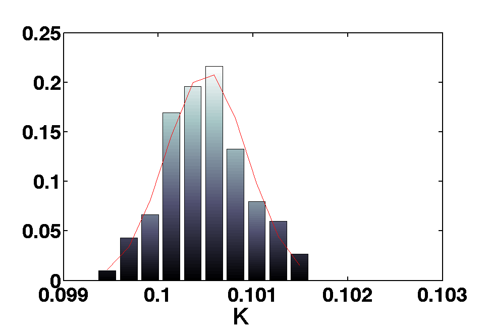
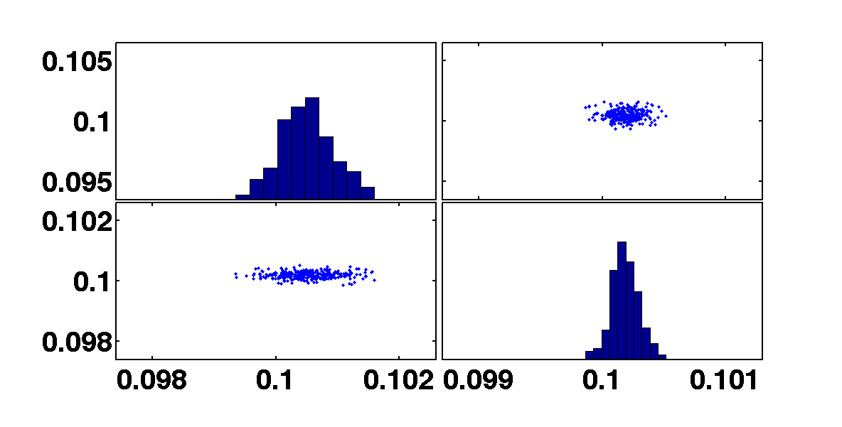
In this simple experiment we use a harmonic oscillator ssm model to simulate date from an input and then we use MCMC to recover the parameters of the model.
    fs    = 10;
    nsecs = 300;
    fin = 0.2

    % Create a sinusoidal input and arrange it to matrix object
    in = ao(plist('waveform', 'sine wave', 'fs', fs, 'nsecs', nsecs, 'f', fin);
    min = matrix(in,plist('shape',[1 1]));
    % we do the same for the noise.
    ns = ao(plist('waveform', 'noise', 'sigma', 0.1, 'nsecs', nsecs, 'fs', fs));
    mnoise = matrix(ns,plist('shape',[1 1]))
    % declare some variables here
    damp = 0.1;
    k = 0.1;
    values = [k , damp];

    % define inNames  and outNames for ssm model. Also declare parameters to be fitted.
    inNames = {'COMMAND.force'};
    outNames = {'HARMONIC_OSC_1D.position'};
    params = {'DAMP','K'};

    % The model to simulate the inputs specified above.
    mod = ssm(plist('built-in','HARMONIC_OSC_1D',...
    'Version','Fitting',...
    'Continuous',1,...
    'SYMBOLIC PARAMS',params));

    % Set the parameters k and damp to the ssm model.
    mod.setParameters(plist('names',params,'values',values));

    % Modify time step and make the model numerical.
    mod.modifyTimeStep('newtimestep', 0.1);

    % Generate covariance
    mod.generateCovariance;

    % Simulate the output after defining the plist.
    pl = plist('Nsamples', fs*nsecs, ...
    'aos variable names',{'COMMAND.force' 'NOISE.readout'},...
    'aos', [in ns],...
    'return outputs', outNames,...
    'cpsd variable names', cov.find('names'), ...
    'cpsd', cov.find('cov'), ...
    'displayTime', true);

    out = mod.simulate(pl);
    model = ssm(plist('built-in','HARMONIC_OSC_1D',...
    'Version','Fitting',...
    'Continuous',1,...
    'SYMBOLIC PARAMS',params));
    % if we type model in the terminal we will see
    % all the information available for the model we just created

    M:   running display
    ------ ssm/1 -------
    amats: {  [2 x2 ]  }  [1x1]
    bmats: {  [2 x1 ]    []    }  [1x2]
    cmats: {  [1 x2 ]  }  [1x1]
    dmats: { [0] [1] }  [1x2]
    timestep: 0
    inputs:  [1x2 ssmblock]
    1 : COMMAND | force [kg m s^(-2)]
    2 : NOISE | readout [m]
    states:  [1x1 ssmblock]
    1 : HARMONIC_OSC_1D | x [m], xdot [m s^(-1)]
    outputs:  [1x1 ssmblock]
    1 : HARMONIC_OSC_1D | position [m]
    numparams: (M=1)
    params: (K=1, DAMP=1)
    Ninputs: 2
    inputsizes: [1 1]
    Noutputs: 1
    outputsizes: 1
    Nstates: 1
    statesizes: 2
    Nnumparams: 1
    Nparams: 2
    isnumerical: false
    hist: ssm.hist
    procinfo: []
    plotinfo: []
    name: HARMONIC_OSC_1D
    description: Harmonic oscillator
    mdlfile:
    UUID: b94172bc-9851-42cd-b56a-ca05503165ad
    --------------------
    ranges = [1e-8 1e-8 ;
    0.5  0.5];

    pl = plist('FitParams',params,...
    'paramsValues',values,...
    'inNames',inNames,...
    'ngrid',20,...
    'stepRanges',ranges,...
    'outNames',outNames,...
    'noise',mnoise,...
    'f1',1e-4,...
    'f2',1,...
    'model',mod,...
    'Navs',5,...
    'pinv',false);

    mcrb = crb(min,pl);
    % First define some variables.
    c = 1;
    ranges = {[-3 3] [-3 3]};
    h = 3;
    Tc = [20 80];
    numsampl = 200;

    % Then we create the plist for the mcmc.
    pl = plist('N',numsampl,...
    'J',1,...
    'cov',c*mcrb.y,...
    'range',ranges,...
    'Fitparams',params,...
    'input',min,...
    'noise',mnoise,...
    'model',model,...
    'inNames',inNames,...
    'outNames',outNames,...
    'frequencies',[1e-4 0.5],...
    'fsout',0.2,...
    'Navs',5,...
    'search',true,...
    'Tc',Tc,'heat',h,...
    'jumps',[2e0 1e1 5e2 1e3],...
    'x0',values,...
    'simplex',false);

    [b smplr]= mcmc(out,pl);
There is also the possibility to use a desired proposal distribution. The user may choose to draw samples from a distribution that is well fitted to the current investigation. An example is shown below:
% Suppose that we want to investigate the same problem as above.
% The plist now should include some extra parameters:

% First of all the function that draws the samples from the
% desired distribution. It must be based on the covariance matrix and
% the current position of the chain mu. For example:
propsamp = @(mu,cov) drawSamplesFromMySampler(arg1,arg2,...,mu,cov);

% Secondly, if the proposal PDF is not symmetric, we should add a function
% that calculates the probability density on the new point x.
% If left empty, then symmetricity is assumed
propdpf = @(x,mu,cov) calcDensityFromMyPDF(x,mu,cov,arg1,arg2,...,argN);

    pl = plist('N',numsampl,...
    'J',1,...
    'cov',c*mcrb.y,...
    'range',ranges,...
    'Fitparams',params,...
    'input',min,...
    'noise',mnoise,...
    'model',model,...
    'inNames',inNames,...
    'outNames',outNames,...
    'proposal sampler',propsamp,...
    'proposal pdf',propdpf,...
    'frequencies',[1e-4 0.5],...
    'fsout',0.2,...
    'Navs',5,...
    'search',true,...
    'Tc',Tc,'heat',h,...
    'jumps',[2e0 1e1 5e2 1e3],...
    'x0',values,...
    'simplex',false);
| |
Markov Chain Monte Carlo | Linear Parameter Estimation with Singular Value Decomposition | |
©LTP Team