LTPDA Toolbox™

Discrete Derivative

Derivative calculation for dicrete data series

Derivative estimation on discrete data series is implemented by the function ao/diff. This function embeds several algorithms for the calculation of zero, first and second order derivative. Where with zero order derivative we intend a particular category of data smoothers [1].

Algorithm

Method	Description
'2POINT'	Compute first derivative with two point equation according to:
'3POINT'	Compute first derivative with three point equation according to:
'5POINT'	Compute first derivative with five point equation according to:
'FPS'	Five Point Stencil is a generalized method to calculate zero, first and second order discrete derivative of a given time series. Derivative approximation, at a given time t = kT (k being an integer and T being the sampling time), is calculated by means of finite differences between the element at t with its four neighbors: It can be demonstrated that the coefficients of the expansion can be expressed as a function of one of them [1]. This allows the construction of a family of discrete derivative estimators characterized by a good low frequency accuracy and a smoothing behavior at high frequencies (near the nyquist frequency). Non-trivial values for the 'COEFF' parameter are: Parabolic fit approximation These coefficients can be obtained by a parabolic fit procedure on a generic set of data [1]. Zeroth order -3/35 First order -1/5 Second order 2/7 Taylor series expansion These coefficients can be obtained by a series expansion of a generic set of data [1 - 3]. First order 1/12 Second order -1/12 PI This coefficient allows to define a second derivative estimator with a notch feature at the nyquist frequency [1]. Second order 1/4

Examples

Consider a as a time series analysis object. First and second derivative of a can be easily obtained with a call to diff. Please refer to ao/diff documantation page for the meaning of any parameter.

Frequency response of first and second order estimators is reported in figures 1 and 2 respectively.

First derivative

    
    pl = plist(...
      'method', '2POINT');
    b = diff(a, pl);
    
    pl = plist(...
      'method', 'ORDER2SMOOTH');
    c = diff(a, pl);
    
    pl = plist(...
      'method', '3POINT');
    d = diff(a, pl);
    
    pl = plist(...
      'method', '5POINT');
    e = diff(a, pl);
    
    pl = plist(...
      'method', 'FPS', ...
      'ORDER', 'FIRST', ...
      'COEFF', -1/5);
    f = diff(a, pl);

Second derivative

    
    pl = plist(...
      'method', 'FPS', ...
      'ORDER', 'SECOND', ...
      'COEFF', 2/7);
    b = diff(a, pl);
    
    pl = plist(...
      'method', 'FPS', ...
      'ORDER', 'SECOND', ...
      'COEFF', -1/12);
    c = diff(a, pl);
    
    pl = plist(...
      'method', 'FPS', ...
      'ORDER', 'SECOND', ...
      'COEFF', 1/4);
    d = diff(a, pl);

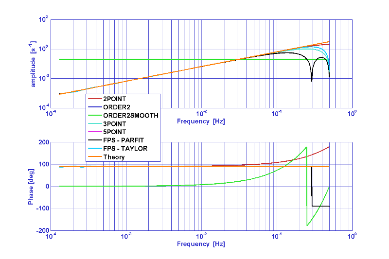
Figure 1: Frequency response of first derivative estimators.

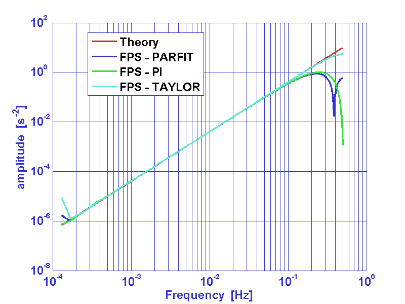
Figure 2: Frequency response of second derivative estimators.

References

L. Ferraioli, M. Hueller and S. Vitale, Discrete derivative estimation in LISA Pathfinder data reduction, Class. Quantum Grav. 26 (2009) 094013..
L. Ferraioli, M. Hueller and S. Vitale, Discrete derivative estimation in LISA Pathfinder data reduction arXiv:0903.0324v1
Steven E. Koonin and Dawn C. Meredith, Computational Physics, Westview Press (1990).
John H. Mathews, Computer derivations of numerical differentiation formulae, Int. J. Math. Educ. Sci. Technol., 34:2, 280 - 287.