By discretizing transfer function models (LTPDA Toolbox)

In the following we want to show how to go from continuous (s) domain to digital (z) domain when working with transfer function models. We will keep working with the models from our previous closed loop example.

Discretizing a transfer function model

Once we have our continuous models it is fairly simple to obtain their digital representation. We can insert them into the miir constructor specifying a sampling frequency, for instance fs = 10 Hz, as follows:

    G_digital = miir(G, plist('fs', 10));
    H_digital = miir(H, plist('fs', 10));
    OLG_digital = miir(OLG, plist('fs', 10));

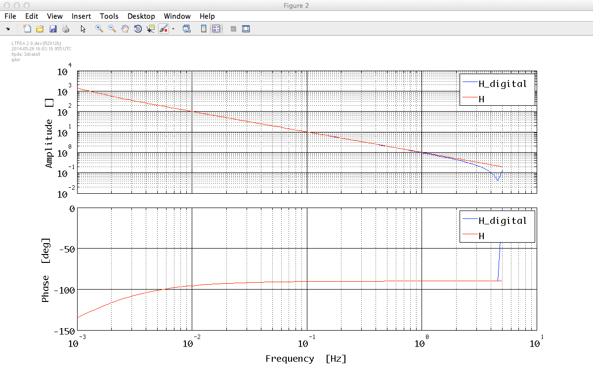
We want to check if the discretization went right, but in order to do that we need to compute the response for the digital and the continuous versions separately, since the resp method can not process inputs from different types. We can do the following:

    %% Compare response

    pl_resp = plist('f1', 1e-3, 'f2', 5, 'nf', 100);

    % Digital
    rG_digital = resp(G_digital, pl_resp);
    rG_digital.setName('G_digital');
    rH_digital = resp(H_digital, pl_resp);
    rH_digital.setName('H_digital');
    rOLG_digital = resp(OLG_digital, pl_resp);
    rOLG_digital.setName('OLG_digital');

    % Continuous
    rG = resp(G, pl_resp);
    rG.setName('G');
    rH = resp(H, pl_resp);
    rH.setName('H');
    rOLG = resp(OLG, pl_resp);
    rOLG.setName('OLG');

    % Plot
    iplot(rG_digital, rG)
    iplot(rH_digital, rH)
    iplot(rOLG_digital, rOLG)

Once the comparison is done, one is usually interested in the coefficients of the digital implementation. These are directly accessible as, for example, Gd.a or Gd.b

    >> Gd.a

    ans =

    3.99874501384116      2.51248480253707e-06         -3.99874250135635

    >> Gd.b

    ans =

    1      0.000628121200622944        -0.999371878799377

The Delay strikes back

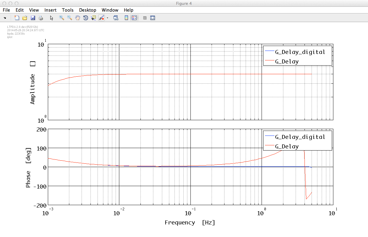
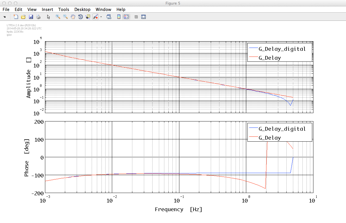
The current version of the toolbox (v2.8) is not able to translate a model with a delay into a digital filter. In such a case, the delay is ignored and a warning is thrown.

     M: running miir/miir
     !!!  PZmodel delay is not used in the discretization

By discretizing transfer function models

By discretizing transfer functions

Discretizing a transfer function model

The Delay strikes back