LTPDA Toolbox™

Topic 4 - Transfer function models and digital filtering

IFO/Temperature Example - Spectral Analysis

Loading the consolidated data sets from topic 2

In the last topic you should have saved your consolidated data files as

ifo_temp_example/temp_fixed.xml
ifo_temp_example/ifo_fixed.xml

In order to proceed with the spectral analysis, we need to use the ao constuctor, with the set of parameters "From XML File". The key parameters are:

Key	Value	Description
`FILENAME`	'ifo_temp_example/ifo_fixed.xml'	The name of the file to read the data from.
`FILENAME`	'ifo_temp_example/temp_fixed.xml'	The name of the file to read the data from.

Hint: the command-line sequence may be similar to the following:

%% Get the consolidated data
% Using the xml format

T_filename = 'ifo_temp_example/temp_fixed.xml';
x_filename = 'ifo_temp_example/ifo_fixed.xml';

pl_load_T = plist('filename', T_filename);
pl_load_x = plist('filename', x_filename);

% Build the data aos
T = ao(pl_load_T);
x = ao(pl_load_x);

Estimating the PSD of the signals

To perform the PSD estimation, you can use the method

ao/lpsd

Hint: the command-line sequence may be similar to the following:

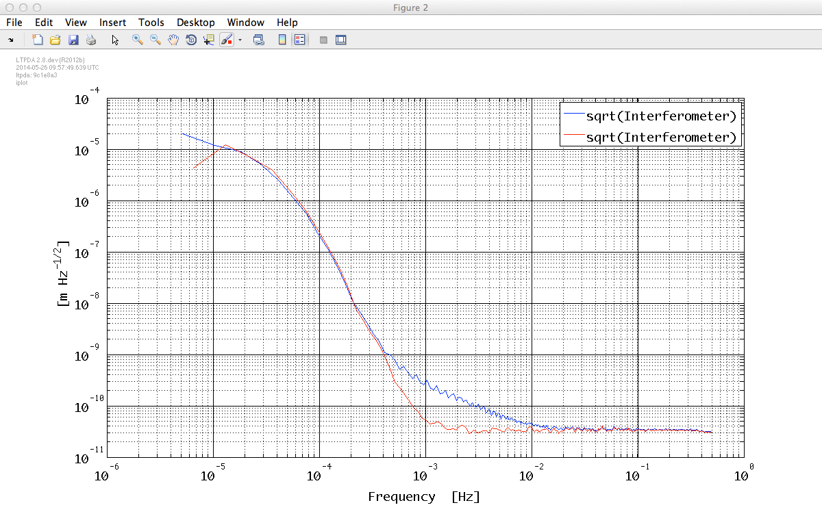
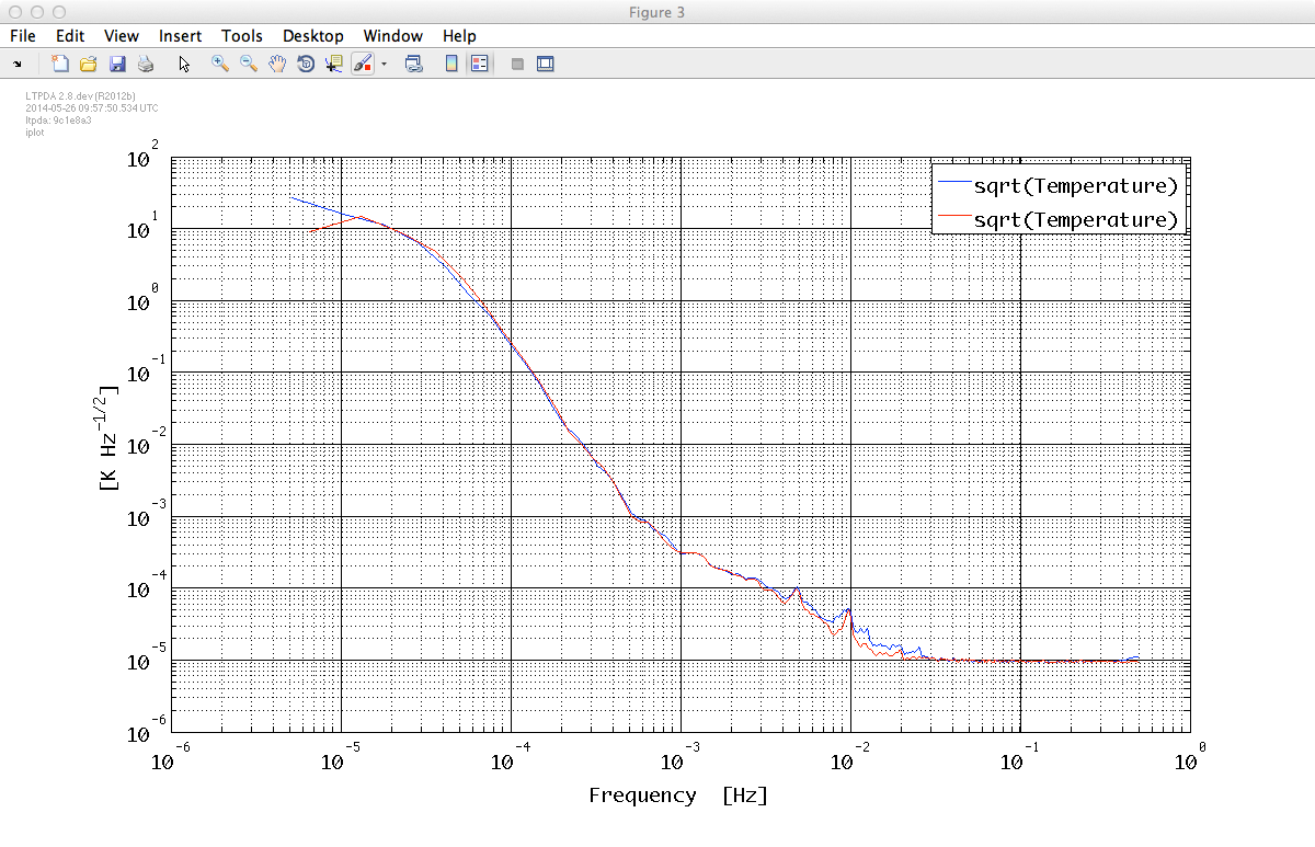
%% PSD
x_psd = lpsd(x)
x_psd.setName('Interferometer');

T_psd = lpsd(T)
T_psd.setName('Temperature');

% Plot estimated PSD
pl_plot = plist('Arrangement', 'subplots', 'LineStyles', {'-','-'},'Linecolors', {'b', 'r'});
iplot(sqrt(x_psd), sqrt(T_psd), pl_plot);

Reducing time interval

Looking at the output of the analysis it is easy to recognize in the IFO PSD the signature of some strong "spike" in the data. Indeed, if we plot the x data, we can find it around t = 40800. There is also a leftover from the filtering process performed during consolidation right near to the last data.

We can then try to estimate the impact of the "glitch" by comparing the results we obtain by passing to ao/lpsd a reduced fraction of the data.

In order to select a fraction of the data we use the method:

ao/split

The relevant parameters for this method are listed here, together with their recommended values:

Key	Value	Description
`SPLIT_TYPE`	'interval'	The method for splitting the `ao`
`START_TIME`	x.t0 + 40800	A time-object to start at
`END_TIME`	x.t0 + 193500	A time-object to end at

Notice that in order to perform this action, we access one property of the ao object, called "t0". The call to the t0 methods gives as an output an object of the time class. Additionally, it's possibly to directly add a numer (in seconds) to obtain a new time object.

Hint: the command-line sequence may be similar to the following:

%% Skip some IFO glitch from the consolidation

pl_split = plist('start_time', x.t0 + 40800, ...
  'end_time', x.t0 + 193500);

x_red = split(x, pl_split);
T_red = split(T, pl_split);

Note: you can also use the parameter 'times' for split to specify times relative to the first sample. In this case:

            plist('times', [40800 193500]).

would work.

And we can proceed, evaluating 2 more aos to compare the effect of skipping the "glitch". After doing that, we can plot them in comparison.

Hint:

%% PSD
x_red_psd = lpsd(x_red);
x_red_psd.setName('Interferometer');

T_red_psd = lpsd(T_red)
T_red_psd.setName('Temperature');

% Plot estimated PSD
pl_plot = plist('Arrangement', 'stacked', 'LineStyles', {'-','-'},'Linecolors', {'b', 'r'});
iplot(sqrt(x_psd), sqrt(x_red_psd), pl_plot);
iplot(sqrt(T_psd), sqrt(T_red_psd), pl_plot);

Estimating the cross-spectra

We can now proceed and use the

ao/lcpsd

method to evaluate the cross-spectra of the signals, employing a shorter window in order to reduce the scatter of the estimated values.

Hint:

%% CPSD estimate
CTx = lcpsd(T_red, x_red);
CxT = lcpsd(x_red, T_red);

% Plot estimated CPSD
iplot(CTx);
iplot(CxT);

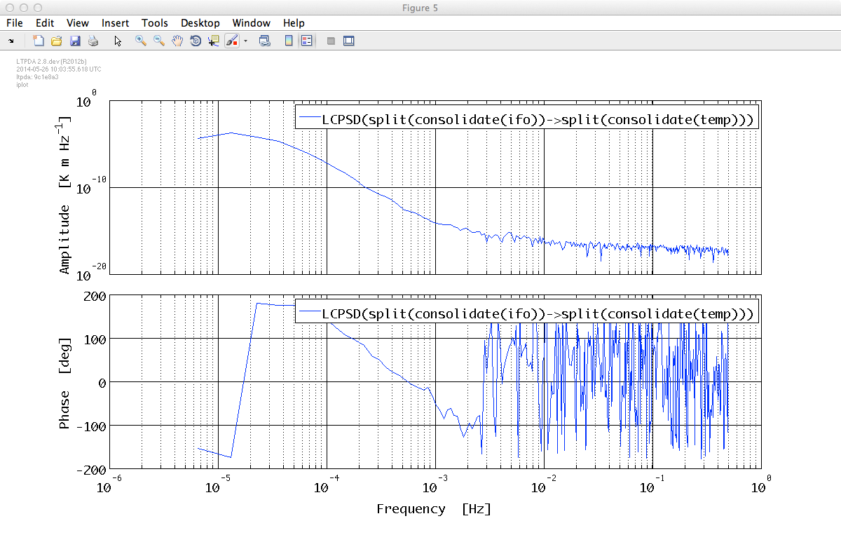
As expected, there is a strong low-frequency correlation between the IFO data x and the temperature data T.

Estimating the cross-coherence

Similarly, we can now proceed and use the

ao/lcohere

method to evaluate the cross-coherence of the signals. The output will be a [2x2] matrix of aos, and we want to look at one of the off-diagonal terms:

%% Coherence estimate
coh = lcohere(T_red, x_red);
      
% Plot estimated cross-coherence
iplot(coh, plist('YScales', 'lin'))

The coherence approaches 1 at low frequency.

Estimating the transfer function of temperature

We want now to perform noise projection, trying to estimate the transfer function of the temperature signal into the interferometer output. In order to do that, we can use the

ao/ltfe

method.

We also want to plot this transfer function to check that the units are correct.
Hint:

%% transfer function estimate
tf = ltfe(T_red, x_red)

% Plot estimated TF
iplot(tf);

As expected, the transfer function T -> IFO is well measured at low frequencies.

Noise projection

We can eventually perform the noise projection, estimating the amount of the noise in the IFO being actually caused by temperature fluctuations. It's a frequency domain estimate:

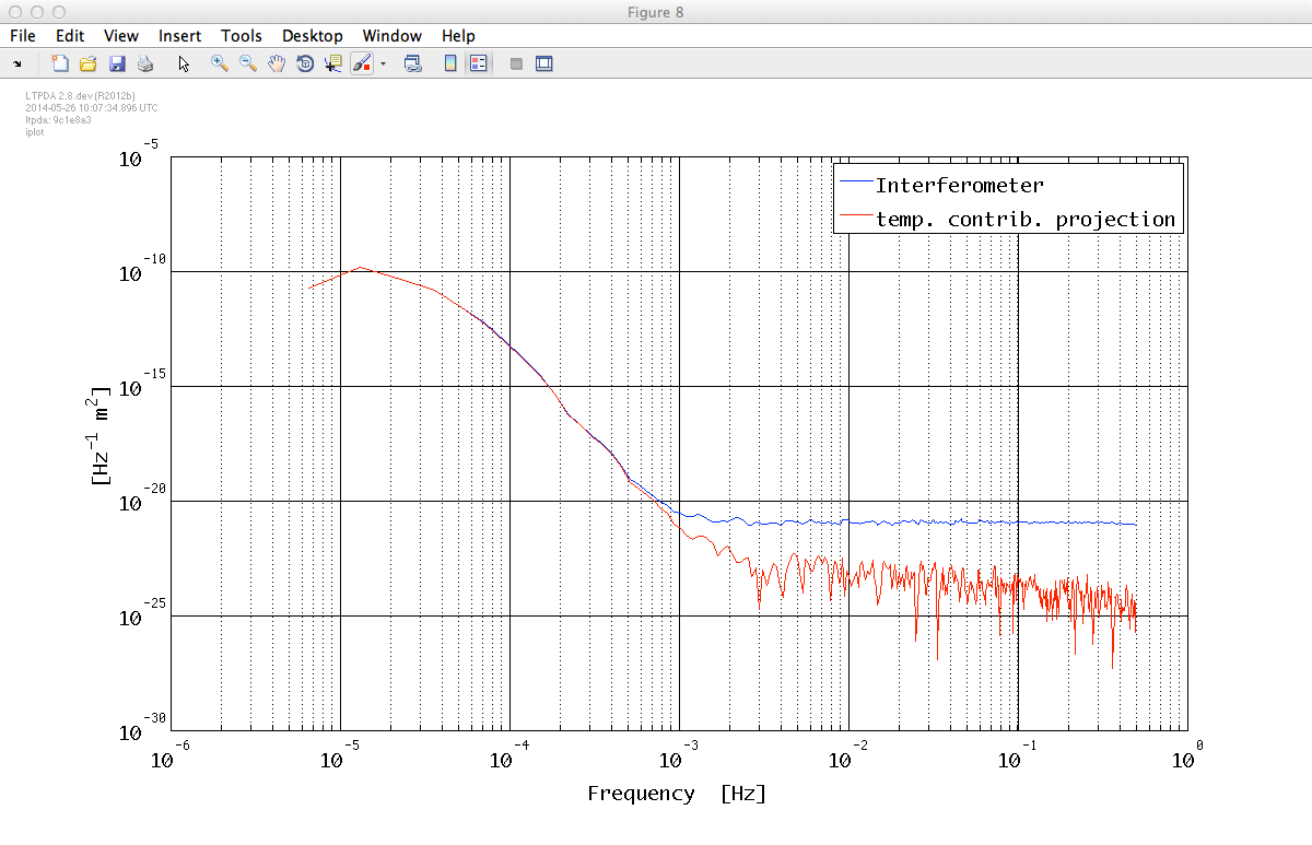
%% Noise projection in frequency domain

proj = T_red_psd .* (abs(tf)).^2;
proj.simplifyYunits;
proj.setName('temp. contrib. projection')

%% Plotting the noise projection in frequency domain
iplot(x_red_psd, proj);

The contribution of the temperature fluctuations is clearly estimated.

Saving the results

Let's fininsh this section of the exercise by saving the results on disk, in xml or mat format. We want to keep the results about the Power Spectral Density and Transfer Function Estimates, at least.

Hint: the command-line sequence may be similar to the following:

%% Save the PSD data
% xml format

pl_save_x_PSD = plist('filename', 'ifo_temp_example/ifo_psd.xml');
pl_save_T_PSD = plist('filename', 'ifo_temp_example/T_psd.xml');

pl_save_xT_CPSD = plist('filename', 'ifo_temp_example/ifo_T_cpsd.xml');
pl_save_xT_cohere = plist('filename', 'ifo_temp_example/ifo_T_cohere.xml');

pl_save_xT_TFE = plist('filename', 'ifo_temp_example/T_ifo_tf.xml');

% mat format

pl_save_x_PSD = plist('filename', 'ifo_temp_example/ifo_psd.mat');
pl_save_T_PSD = plist('filename', 'ifo_temp_example/T_psd.mat');

pl_save_xT_CPSD = plist('filename', 'ifo_temp_example/ifo_T_cpsd.mat');
pl_save_xT_cohere = plist('filename', 'ifo_temp_example/ifo_T_cohere.mat');

pl_save_xT_TFE = plist('filename', 'ifo_temp_example/T_ifo_tf.mat');

and

% Save
x_red_psd.save(pl_save_x_PSD);
T_red_psd.save(pl_save_T_PSD);
CxT.save(pl_save_xT_CPSD);
coh.save(pl_save_xT_cohere);
tf.save(pl_save_xT_TFE);

Empirical Transfer Function estimation

Topic 4 - Transfer function models and digital filtering