LTPDA Toolbox™

IFO/Temperature Example - Pre-processing

Now we return to the IFO/Temperature example that was started in Topic 1.

Loading and checking the calibrated data sets from topic2

In the last topic you should have saved your calibrated data files as
ifo_temp_example/ifo_disp.xml and
ifo_temp_example/temp_kelvin.xml

Now load each file into an AO, and simplify the name of the objects by assigning them the name of the Matlab workspace variable containing them:

    ifo  = ao('ifo_temp_example/ifo_disp.xml');
    temp = ao('ifo_temp_example/temp_kelvin.xml');
    ifo.setName;
    temp.setName;

Let's see what kind of pre-processing we have to apply to our data prior to further analysis.

You can have a look at the data by for example displaying the AOs on the terminal and by plotting them, of course. Since the two data series have different Y units, we should plot them on subplots. To do that with iplot, pass the key 'arrangement' in a plist. For example:

    pl = plist('arrangement', 'subplots');

If you plot the two time-series you should see something like the following:
ifotempdata

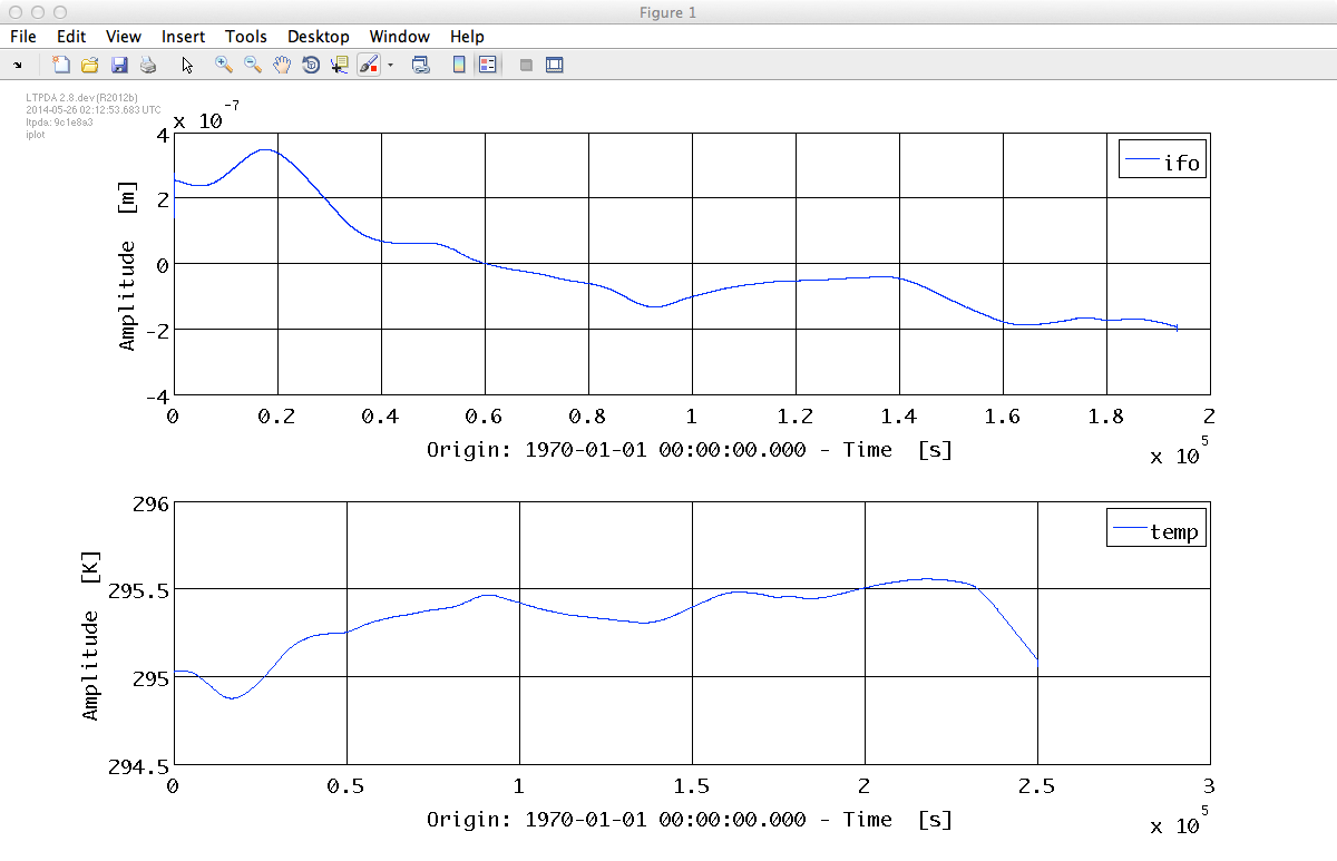
Some points to note:

The two data streams:
- do not have the same sampling frequency.
- are not of the same length (nsecs).
The interferometer data has a small transient at the start

To have a closer look at the samples we plot markers at each sample and only plot a zoomed-in section. You can do this by creating a parameter list with the following key/value pairs (remember the 'key' properties for plist entries is not case sensitive):

Key	Value
`ARRANGEMENT`	'subplots'
`LINESTYLES`	{'none', 'none'}
`MARKERS`	{'+', '+'}
`XRANGES`	{'all', [200 210]}
`YRANGES`	{[2e-7 3e-7], [200 350]}

Notice the use of the keyword 'all' in the value for the 'XRANGES' parameter. Many of the iplot options support this keyword, which tells iplot to use the same value for all plots and subplots. For the 'YRANGES' we specify different values for each subplot.

Please store the parameter lists for plot settings in 2 different variables. We can reuse them for plotting our results later.

Passing such a parameter list to iplot together with the two AO time-series should yield a plot something like:

From this plot you may be able to see that the temperature data is unevenly sampled.

To confirm this, enter the following (standard) MATLAB commands on the terminal:

    dt = diff(temp.x);
    min(dt)
    max(dt)

Don't forget the semicolon at the end of the diff calculation; this is a long data series and will be printed to the terminal if you do forget.

You see that the minimum and maximum difference in the time-stamps of the data is different, showing that the data are not evenly sampled.

Before we proceed with the later analysis of this data, we need to

Fix the uneven sampling of the temperature data
Resample both data streams to the same rate
Resample both data streams on to the same timing grid
Select the segment of interferometer data that matches the temperature data

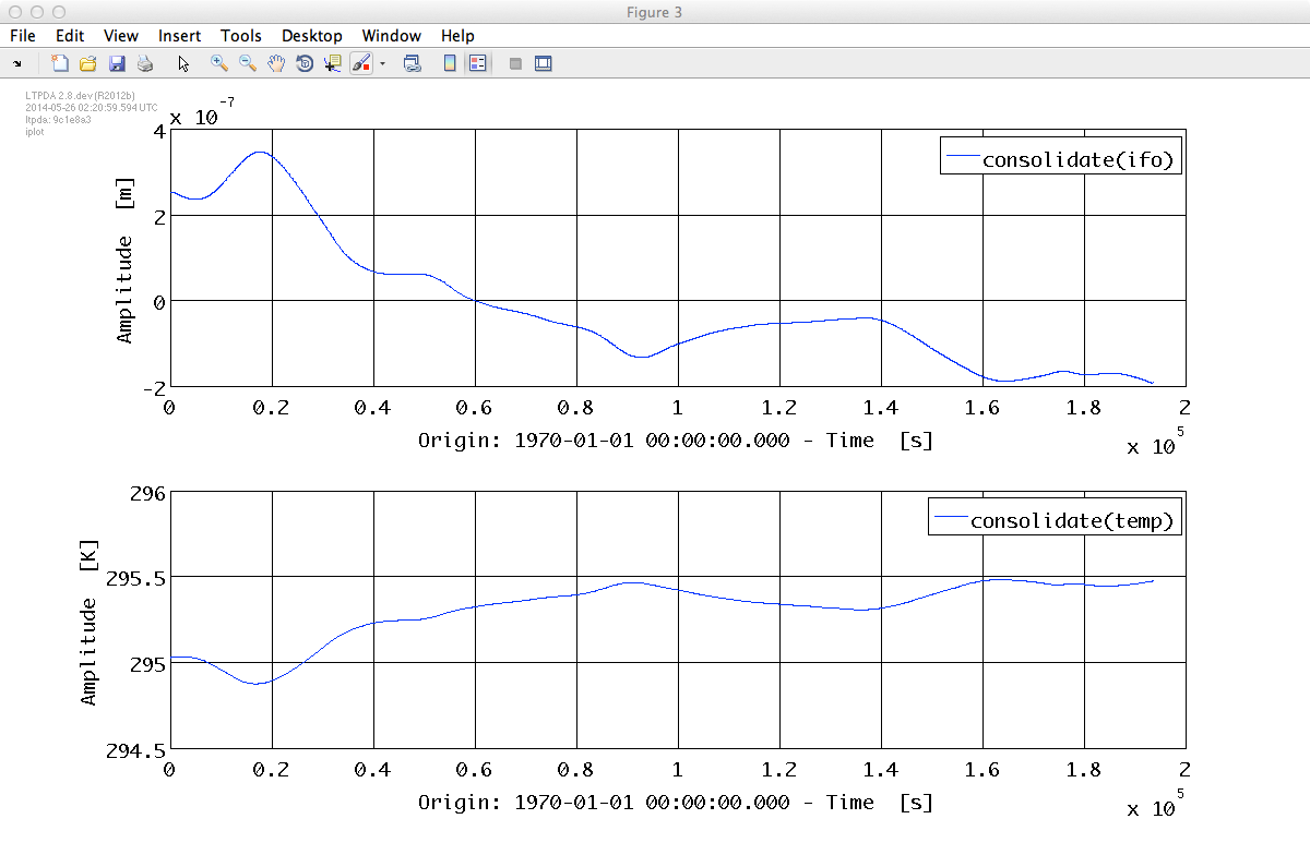
Each of these steps can, in principle, be done by hand. However, LTPDA provides a 'data fixer' method called ao/consolidate which attempts to automate this process. The call to consolidate is shown below:

    [temp_fixed ifo_fixed] = consolidate(temp, ifo, plist('fs', 1));

We tell consolidate that we want to have our data resampled to 1 Hz by specifying the parameter key 'fs'.

Now we can inspect the time-series of these data. The result should look something like the figure below:

If we also plot the zoomed-in view again, we should see something like:

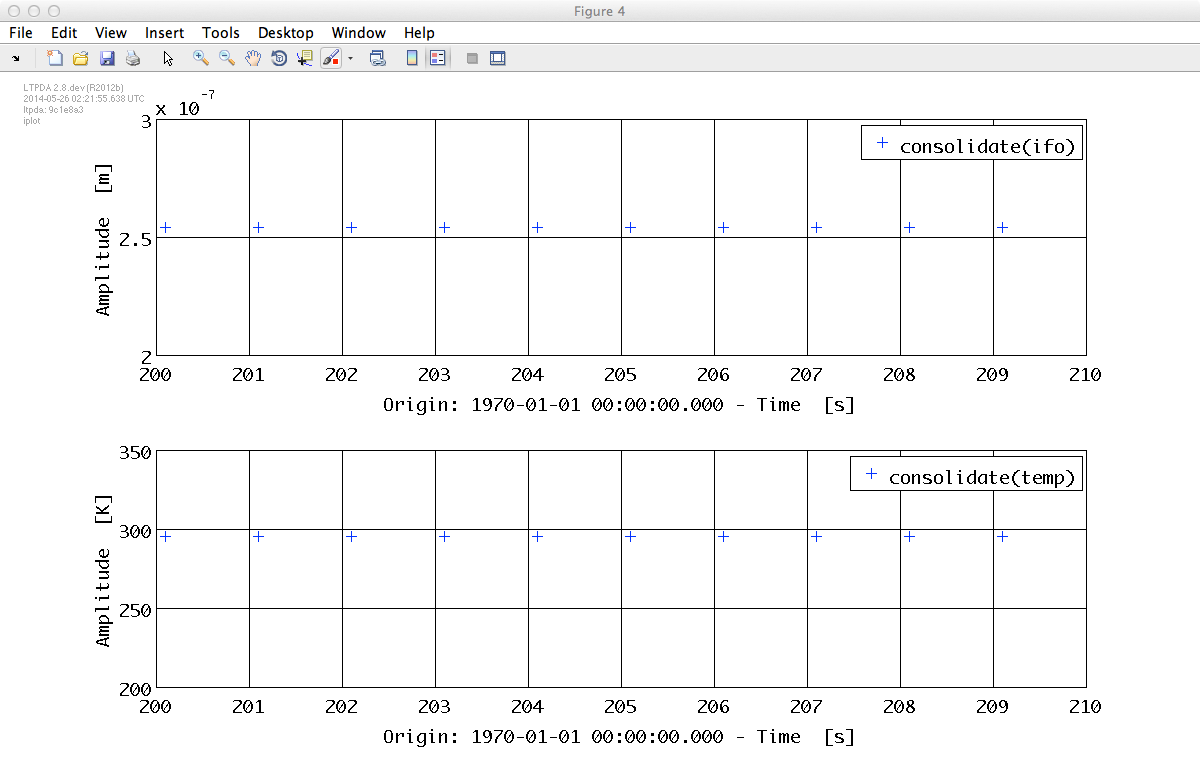
As you can see consolidate solved all our issues with these two data streams. They now start at the same time and are evenly sampled at the same sampling frequency.

In the next topic, we will look at the spectral content and coherence of the data before and after the pre-processing. For now, finish by saving the consolidated data ready for the next topic.

    save(temp_fixed, 'ifo_temp_example/temp_fixed.xml');
    save(ifo_fixed, 'ifo_temp_example/ifo_fixed.xml');

Split and join AOs

Topic 3 - Spectral Analysis