

| LTPDA Toolbox™ | contents | |
Upsampling increases the sampling rate of the input AOs by an integer factor
The ao/upsample method can take the following parameters:
| Key | Description |
|---|---|
|
N |
The upsample factor. The algorithm places 'N-1' zeros between each of the original samples. |
|
PHASE |
This parameter specifies an additional sample offset. The value must be between 0 and N-1. |
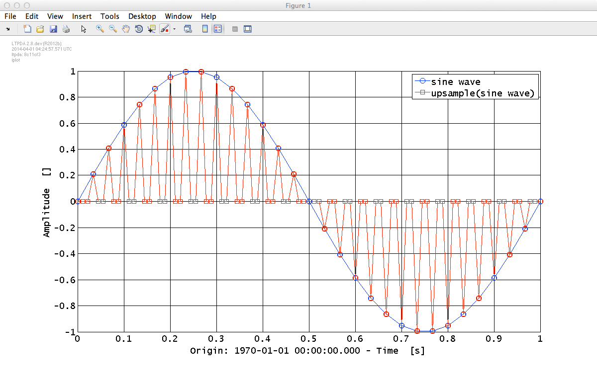
We will upsample a sine-wave by a factor of 3 with no initial phase offset.
Start by creating a sine-wave at 1Hz with a 30Hz sample rate and 10 seconds long. We can use the ao "From Waveform" parameter set to do this. (Equally, we can do this with the "From Time-series Function" parameter set.)
    pl = plist('Waveform', 'sine wave', 'f', 1, 'fs', 30, 'nsecs', 10);
    x  = ao(pl);
Now we can proceed to upsample this data by a factor 3. This will place 2 zero samples between each of the original samples.
    pl_up = plist('N', 3); % increase the sampling frequency by a factor of 10
    x_up  = upsample(x, pl_up); % resample the input AO (x) to obtain the upsampled AO (y)
    iplot(x, x_up, plist('XRanges', [0 1], 'Markers', {'o', 's'})) % plot original and upsampled data
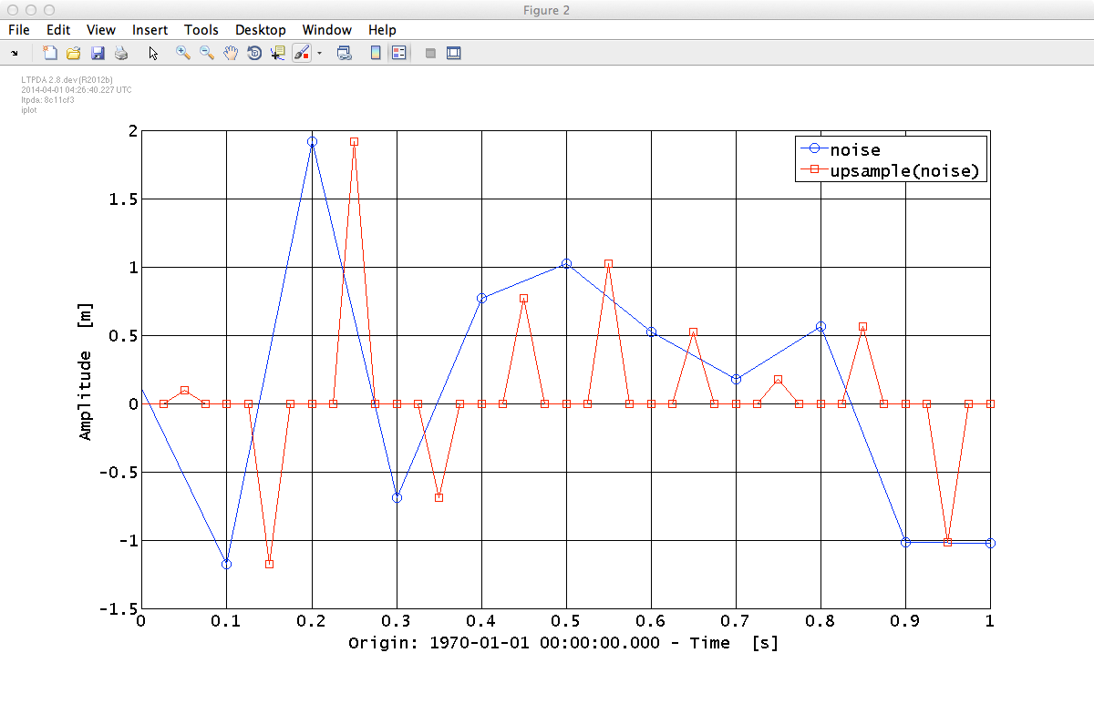
In this second example, we will upsample some random noise by a factor 4 with a phase offset of 2 samples.
Again, start by constructing some test data, in this case a white-noise data stream. We can do this again using the "From Waveform" parameter set with an ao constructor.
pl         = plist('Waveform', 'noise', 'fs', 10, 'nsecs', 10, 'yunits', 'm');
x          = ao(pl);
pl_upphase = plist('N', 4, 'phase', 2); % increase the sampling frequency and add phase of 2 samples to the upsampled data
x_upphase  = upsample(x, pl_upphase); % resample the input AO (x) to obtain the upsampled and delayed AO
iplot(x, x_upphase, plist('XRanges', [0 1], 'Markers', {'o', 's'})) % plot original and upsampled data
| |
Downsampling a time-series AO | Resampling a time-series AO | |
©LTP Team