Parameter estimation with MCMC (LTPDA Toolbox)

At this point we have all the inputs necessary to use the Markoc Chain Monte Carlo. We have the injected signals, the simulated output signals, the covariance matrix of the parameters and the LTP model. First, of course, we load all the objects we created before: the signals and the fitting model.



    
  in    = matrix('input.mat');
  out   = matrix('output.mat');
  noise = matrix('noise.mat');
  mdl   = ssm('fitting_model.mat');

Secondly, we arrange again the parameters to estimate in a cell array and define a vector with their initial values. We also create cell arrays containing the inputs and outputs of the system.




  inNames  = { 'GUIDANCE.IFO_x1'  'GUIDANCE.IFO_x12'};
  outNames = {'DELAY_IFO.x1' 'DELAY_IFO.x12'};

  % Also define again the parameters to estimate and our starting values
  params = {'FEEPS_XX', 'CAPACT_TM2_XX', 'IFO_X12X1', 'EOM_TM1_STIFF_XX', 'EOM_TM2_STIFF_XX'};
  values = [1 1 0.0001 1.e-6 1.e-6];

Now, we have to estimate the expected errors of the parameters based on our first guess of the parameters ([1 1 0.0001 1.e-6 1.e-6]). The covariance matrix extracted from the crb function will be used as the covariance matrix for the proposal distribution of the metropolis algorithm. Just like in section 5.5:


 

   % as in section 5.5 we provide the optimal differentiation step
   steps =  [1e-11 2.3e-07 1e-15 8.4e-11 2.4e-12];
      
   % We define the plist to input to the crb fuction
   % to estimate the errors of the parameters.
   pl_crb = plist('FitParams', params, ...  
              'paramsValues', values, ...         
              'diffStep', steps, ...
              'ngrid', 5 ,...                      % Number of points in the grid to compute the optimal differentiation step for ssm models 
              'inNames', inNames, ...
              'outNames', outNames, ...
              'input', in, ...
              'f1', 1e-4, ...                      % Initial frequency for the analysis
              'f2', 1, ...                         % Final frequency for the analysis
              'model', mdl, ...                   
              'Navs', 5, ...                       % Force number of averages
              'pinv', false);                     % Use the Penrose-Moore pseudoinverse

   % Estimate the CRB
   mcrb = crb(noise, pl_crb);
   
   % Save object
   save(mcrb, 'crb_5params_fitting.mat');

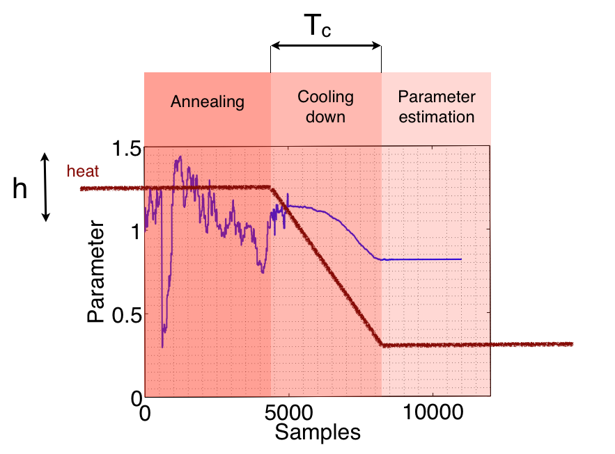
The next step is to call the mcmc method of the LTPDA after we define the input plist. The plist will contain all the settings for the metropolis sampling. There are two parameters which set the main characteristics ot the metropolis algorithm:

Other parameters to be set are: fsout, the desired sampling frequency to resample the input time series or a cell array of ranges for the parameters, meaning the upper and lower bound to search for each one.

 

% Now we define some parameters for the mcmc plist

h = 2;              % heat index for simulated annealing
Tc = [100 1000];    % An array of two values setting the initial 
                    % and final value for the cooling down. We set it to
                    % these values because we use the simplex algorithm
                    % before the sampling and we get close to the real
                    % values. If simplex was set to false then we should set 
                    % Tc = [5000 7000] and 'N' to 9000.
                    
numsampl = 2000;    % Total number of samples

% Upper and lower bounds to search for the parameters 
ranges = {[0 2], [0 2], [0 1], [0 1e-4], [0 1e-4]};

 

  % defining the mcmc plist  
  pl_mcmc = plist('N', numsampl, ...       % Total number of samples
              'J', 1, ...
              'cov', mcrb, ...                 
              'range', ranges, ...
              'FitParams', params, ...            
              'input', in, ...
              'noise', noise, ...
              'model', mdl, ...
              'inNames', inNames, ...
              'outNames', outNames, ...
              'frequencies', [1e-4 0.5], ... 
              'Navs', 5, ...
              'search', true, ...
              'x0', values, ...
              'Tc', Tc, ...
              'heat', h, ...
              'jumps', [2e0 1e2 1e3 1e4], ...
              'simplex', true, ...    % Set simplex to true for speed!
              'plot', [1 2 3 4 5 6], ...
              'debug', false);
  
% start the mcmc sampling and create a new pest object b  
b = mcmc(out, pl_mcmc);

Parameter estimation with MCMC

A) Markov Chain Monte Carlo