

| LTPDA Toolbox™ | contents | |
Injecting signals in to ssm models is done at the time of simulating. In Topic 2 you learned how to simulate an LPF model which generated its noise internally. But you can also inject time-series data into the simulation in the form of AOs.
The two key parameters for ssm/simulate are:
| Key | Description |
|---|---|
| AOS | An array of AOs to be input to the simulation. Specify one per ''AOS VARIABLE NAMES''. |
| AOS VARIABLE NAMES | An cell-array of strings which give the names of the input ports you want to inject the AOs into. |
	  % The following supposes you already have an LPF SSM model called 'lpf' in your MATLAB workspace.

      % Create some time-series analysis object to inject
      aSignal = ao(plist('tsfcn', '1e-6*sin(2*pi*0.1*t)', 'fs', 10, 'nsecs', 1000));

      % Create the plist to configure simulate
      sim_pl = plist('AOS', aSignal, 'AOS Variable Names', 'GUIDANCE.ifo_x1', 'return outputs', 'DELAY_IFO.x1')

      % Run the simulation
      out = simulate(lpf, sim_pl);
      % The following supposes you already have an LPF SSM model called 'lpf' in your MATLAB workspace.

      % Create some time-series analysis object to inject
      fs    = 1/lpf.timestep; % Get the sample rate from the model's timestep
      nsecs = 1000; % Create signals 1000s long
      sig1 = ao(plist('tsfcn', '1e-6*sin(2*pi*0.1*t)', 'fs', fs, 'nsecs', nsecs));
      sig2 = ao(plist('built-in', 'signals_3045_1_1', 'gaps', 1000));

      % Create the plist to configure simulate
      sim_pl = plist('AOS', [sig1 sig2], ...
                     'AOS Variable Names', {'GUIDANCE.ifo_x1', 'GUIDANCE.ifo_x12'}, ...
                     'return outputs', {'DELAY_IFO.x1', 'DELAY_IFO.x12'})

      % Run the simulation
      out = simulate(lpf, sim_pl);
There are a number of rules which need to be followed for this all to work:
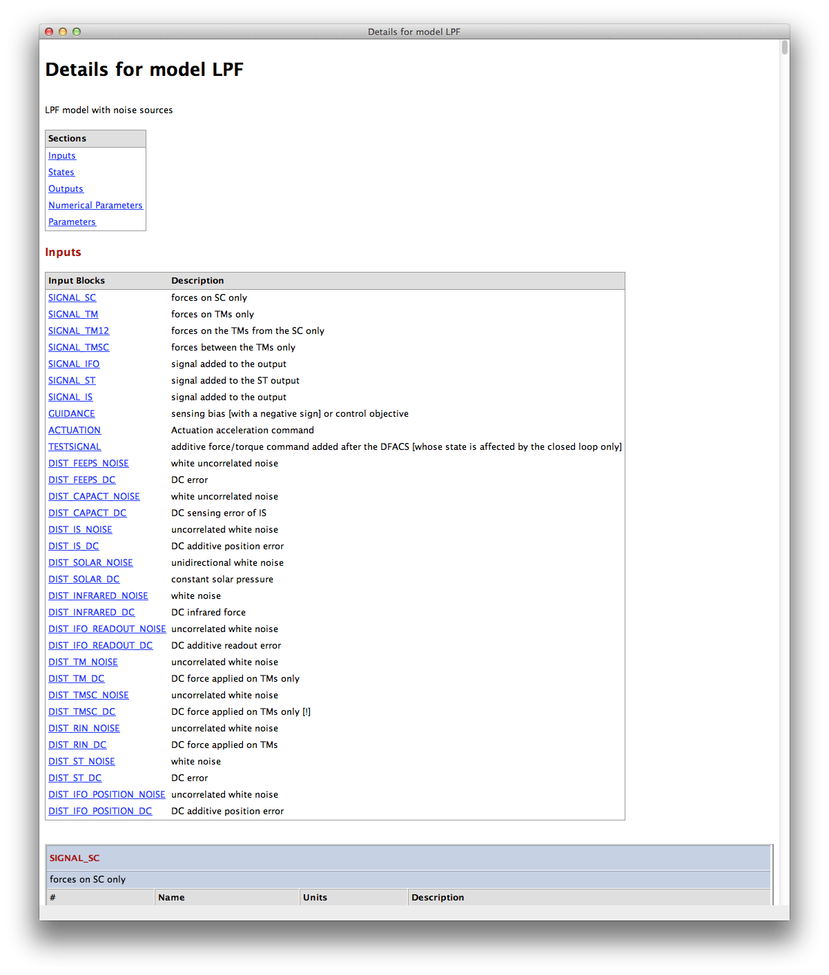
One of the difficulties of working with very large models like the LPF model, is that it's sometimes difficult to see which inputs and outputs are available to you. To aid in this process, we have two tools which can be useful. The first presents details of a given model in a documentation window. For example, suppose we have our LPF model in the MATLAB workspace, then you can do
lpf.viewDetails
portNames = lpf.getPortNamesForBlocks('GUIDANCE');
lpf.getPortNamesForBlocks(plist('blocks', 'guidance', 'type', 'inputs'))
| |
Building signals | Simulate LTP with injected signals (no noise) | |
©LTP Team