

| LTPDA Toolbox™ | contents | |
This exercise starts with the generation of simulated noise data.
    % set output names
    outNames = {...
      'DELAY_IFO.x1'  ...      % o1 IFO
      'DELAY_IFO.x12' ...      % o12 IFO
      'DFACS.sc_x', ...        % Commanded force F_cmd_X
      'DFACS.tm2_x' ...        % Commanded force F_cmd_x2
      };

    % Define parameters and nominal values
    params = {...
      'FEEPS_XX', ...         % FEEPs actuation gain
      'CAPACT_TM2_XX', ...    % Capacitive actuation gain
      'IFO_X12X1', ...        % The coupling of the x position of TM1 to the estimated x position of TM2
      'EOM_TM1_STIFF_XX', ... % Total stiffness of TM1 along X
      'EOM_TM2_STIFF_XX' ...  % Total stiffness of TM2 along X
      };

    % set parameters values for the conversion to acceleration
    FEEPS_XX         = 1;
    CAPACT_TM2_XX    = 1;
    IFO_X12X1        = 1e-4;
    EOM_TM1_STIFF_XX = 1.3e-6;
    EOM_TM2_STIFF_XX = 2.0e-6;

    % actual values for the parameters
    values = [...
      FEEPS_XX, ...
      CAPACT_TM2_XX, ...
      IFO_X12X1, ...
      EOM_TM1_STIFF_XX, ...
      EOM_TM2_STIFF_XX];

    % Create LPF SSM model
    pl = plist('built-in', 'LPF', ...
      'DIM', 1, ...                    % We use a one dimensional model
      'CONTINUOUS', false, ...         % The model is discrete
      'param names', params, ...       % Parameter names
      'param values', values, ...      % Parameter values
      'VERSION', 'Best Case June 2011'); % Model version

    LPF = ssm(pl);

    % Create default noise covariance, assumes independent noise sources
    cov = LPF.generateCovariance;

    % Create a plist to configure the simulation
    plsim = plist(...
              'return outputs', outNames,...
              'cpsd variable names', cov.find('names'), ...
              'cpsd', cov.find('cov'), ...
              'Nsamples', 1e6);

    % Run the simulation
    out = LPF.simulate(plsim);

    % Unpack the signals from the simulation output matrix
    [o1, o12, F_cmd_X, F_cmd_x2] = unpack(out);
Since the method for the conversion to acceleration uses a different naming convention for the parameters, it is convenient to set the convention mapping for the parameters.
    Gdf  = FEEPS_XX;
    Gsus = CAPACT_TM2_XX;
    SD1  = IFO_X12X1;
    w1   = -1*EOM_TM1_STIFF_XX;
    w2   = -1*EOM_TM2_STIFF_XX;
Note that in the method for the conversion to acceleration the stiffness is negative!
'ltp_ifo2acc' likes to work with SI units and in particular the force units have to be expressed in 'kg m s^(-2)'.
    F_cmd_X.toSI;
    F_cmd_x2.toSI;
Now we can set the parameter list for the conversion to acceleration.
    pli2a = plist(...
       'SD1', SD1,...
       'Gdf', Gdf,...
       'Gsus', Gsus,...
       'w1', w1,...
       'w2', w2,...
       'OMS delay o1', 0.3, ...
       'OMS delay oD', 0.3, ...
       'Hdf', F_cmd_X*(-1),...
       'Hsus', F_cmd_x2*(-1)...
      );
Note the -1 multiplying the commanded forces, this is need because of a difference of convention between 'ssm' and 'ltp_ifo2acc' on the controllers outputs.
Now the conversion to equivalent residual acceleration of the interferometer displacement signals.
M = ltp_ifo2acc(o1, o12, pli2a); % M is a matrix object containing a1 and a12
Calculate the square root of the power spetral density in order to check the resuls.
    plpsd = plist(...
      'order', 1, ...
      'SCALE', 'ASD' ...
      );

    Mxx  = M.lpsd(plpsd);
Remove the first 6 samples (lowest frequencies bins) since they are corrupted by the window function.
    plsp = plist(...
      'samples', [7 inf] ...
      );

    Mxxs  = Mxx.split(plsp);
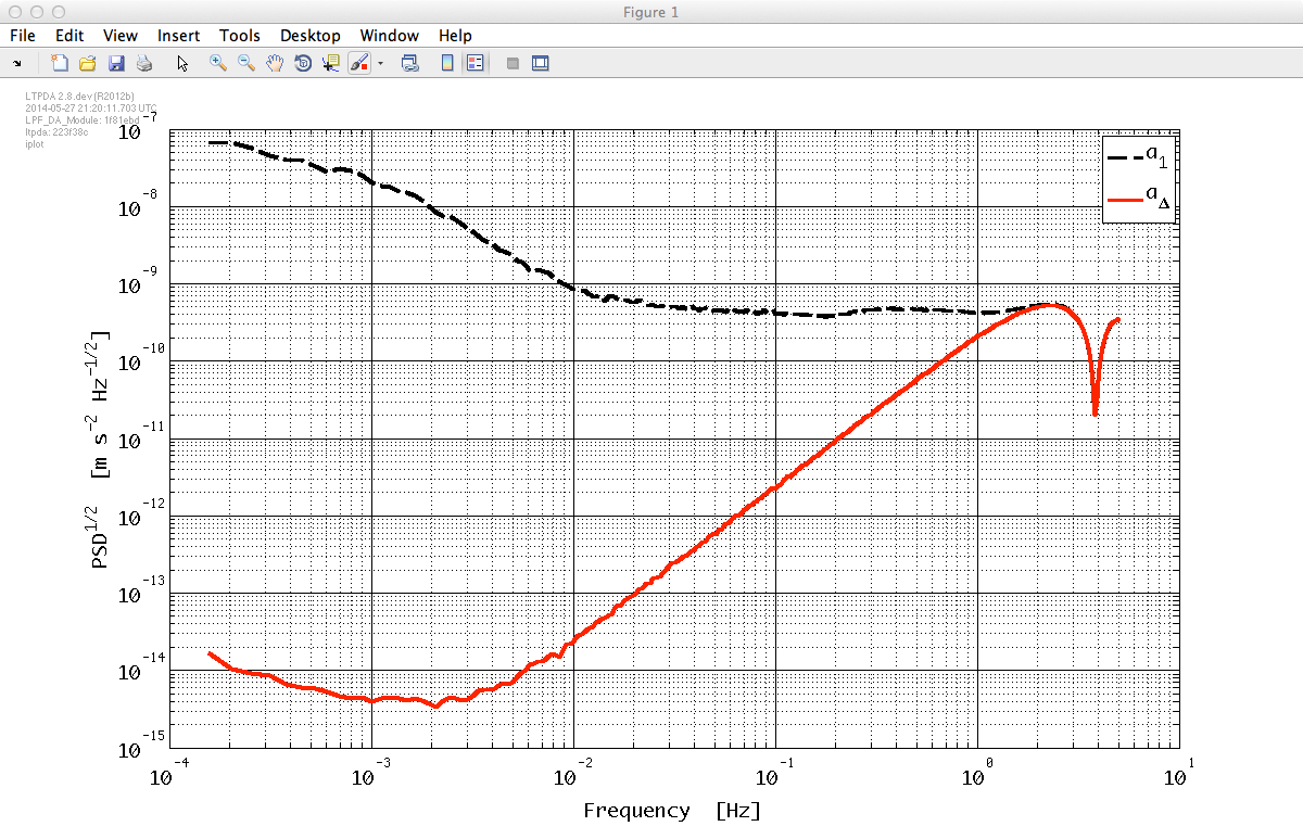
Finally, plot the result.
    plplot = plist(...
    'Linecolors', {'k', 'r'}, ...
    'LineStyles', {'--', '-'}, ...
    'LineWidths', {3, 3}, ...
    'Legends', {'a_1', 'a_{\Delta}'}, ...
    'XLABELS', {'All', 'Frequency'}, ...
    'YLABELS', {'All', 'PSD^{1/2}'} ...
    );


  iplot(Mxxs, plplot)
| |
Tools for estimating the equivalent acceleration in LTPDA | Topic 4 - Simulating LPF with injected signals. | |
©LTP Team