Building an LTP model
Building the LTP model is straightforward. It is simply another built-in model
of the ssm class. Here's an example of building the default version
of the LTP model:
ltp = ssm(plist('built-in', 'LTP'));
To see what other versions of the LTP model are available, and the parameters that can be adjusted,
you can look at the model documentation:
then click on the 'Model Information' link to open a documentation window
like the one shown here:
As you can see, there are various 'Versions' of the model available. Each version
uses different versions of the various submodels, and different default values of the parameters.
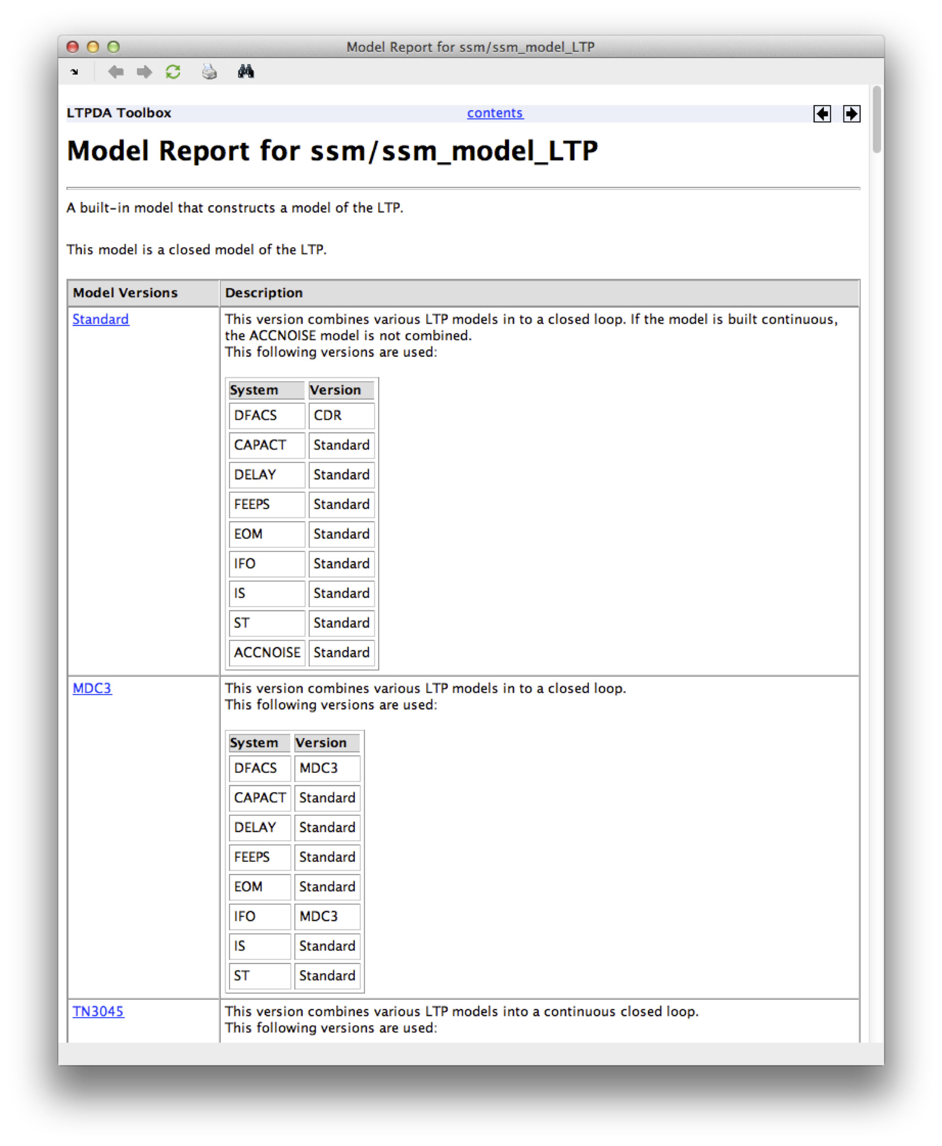
The default version is always the first one!
|
In addition, you can scroll to the
details section for a particular model version and see what configuration parameters
are available to you.
Since the LTP model is assembled from sub-models, it is possible, for each version of the LTP model,
to click on the name of the sub-models to access the documentation window associated with sub-model itself.
For example, we could build a version of the LTP model which is 1D and has DFACS
set to Science Mode 2.2. To do that, you would do:
modelPlist = plist(...
'built-in', 'LTP', ...
'Version', 'Standard', ...
'DIM', 1, ...
'DFACS Mode', 'SCI2.2 M1' ...
);
ltp = ssm(modelPlist);
To look at the details of the model you've built, you can either enter the variable name
on the MATLAB terminal without a terminating semicolon and hit enter. Or, more effectively, you can use the ssm/viewDetails method which will display details
of the model you've constructed in a documentation window:
|
Introduction to the LPF state-space models in LTPDA |
|
Introduction to the various LPF noise models |
 |
©LTP Team