Plotting Analysis Objects (LTPDA Toolbox)

The iplot method provides an advanced plotting interface for AOs which tries to make good use of all the information contained within the input AOs. For example, if the xunits and yunits fields of the input AOs are set, these labels are used on the plot labels.

In addition, iplot can be configured using a input plist. The following examples show some of the possible ways to use iplot

    >> a1 = ao(plist('tsfcn', 'sin(2*pi*0.3*t) + randn(size(t))', 'fs', 10, 'nsecs', 20))
    ----------- ao 01: a1 -----------
 
       name: ''
       data: (0,0.879837752535385) (0.1,2.69334087256333) (0.2,0.840912545780978) (0.3,-0.632154874569397) (0.4,3.00319540765713) ...
             -------- tsdata [x, y] --------
              
                  x:  [200 1], double
                  y:  [200 1], double
                 dx:  [0 0], double
                 dy:  [0 0], double
             xunits:  [s]
             yunits:  
                  fs:  10
               nsecs:  20
                  t0:  1970-01-01 00:00:00.000 UTC
             -------------------------------
              
       hist: ao / ao / 11c33bf1421898d27b94853f646e22673ebc750d
description: 
       UUID: c77f4210-e51d-4240-9a51-276e3f65cc46
---------------------------------

Creates a time-series AO. If we look at the data object contained in this AO, we see that the xunits are set to the defaults of seconds [s].

If we plot this object with iplot we see these units reflected in the x and y axis labels.

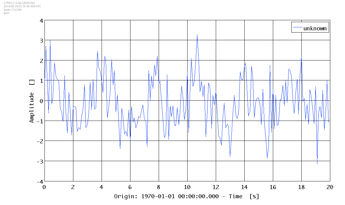
We also see that the time-origin of the data (t0 field of the tsdata class) is displayed as the plot title.